MIT 6.S184 - Lecture 2 - Constructing a Training Target
- Lecture introduction and problem statement
- Class outline and the six central objects (conditional vs marginal)
- Probability path concept and conditional probability path
- Marginal probability path and its density formula
- Conditional vector field and ODE construction per data point
- Marginal vector field and the marginalization trick
- Continuity equation and its role in proving marginalization
- Proof sketch: deriving the marginal continuity equation from conditional dynamics
- Visualization and intuition for flows mapping noise to data
- Score functions: conditional and marginal definitions and relation
- SDE extension (score correction) and the extension trick
- Practical implications, training target and course wrap-up
Lecture introduction and problem statement
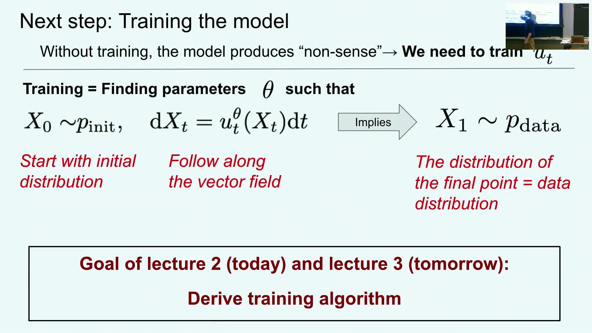
The lecture introduces flow and diffusion generative models and frames sampling as integrating either an ordinary differential equation (ODE) or a stochastic differential equation (SDE) from a simple initial distribution to the data distribution.
- Sampling is described as simulating an ODE/SDE from time 0 to 1 starting from a simple initial law (e.g., isotropic Gaussian).
- The central training problem is to derive a suitable training target for the vector field (drift) so that samples at the terminal time follow the data distribution.
- Untrained models output arbitrary samples, so the core technical question is: how do we construct a loss/target that, when minimized, yields a vector field whose induced endpoint distribution matches the data?
The lecture separates two distinct concerns:
-
Sampling mechanics — how to simulate an ODE/SDE from t=0 to t=1 to produce samples.
-
Learning objectives — what target should the network predict (the vector field, the score, or related conditional quantities).
This distinction motivates the derivations that follow, which derive the conditional and marginal objects used as training targets.
Class outline and the six central objects (conditional vs marginal)
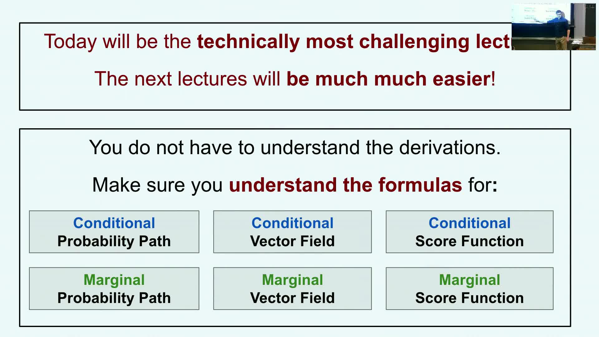
The plan is to derive the marginal vector field and the marginal score, and to emphasize six central mathematical objects:
- Three conditional objects (defined per data point z):
-
Conditional probability path — p_t(x z) - Conditional vector field — u_t(x; z)
-
Conditional score — s_t(x; z)
-
- Three marginal objects (obtained by averaging over the data distribution):
- Marginal probability path — p_t(x)
- Marginal vector field — v_t(x)
-
Marginal score — s_t(x)
Terminology: “conditional” refers to constructs for a fixed data sample z (per data point). “Marginal” denotes the corresponding quantity after marginalizing z under the data distribution p_data(z).
Understanding the definitions and explicit formulas for these six objects is the primary technical requirement for later algorithmic development.
Probability path concept and conditional probability path
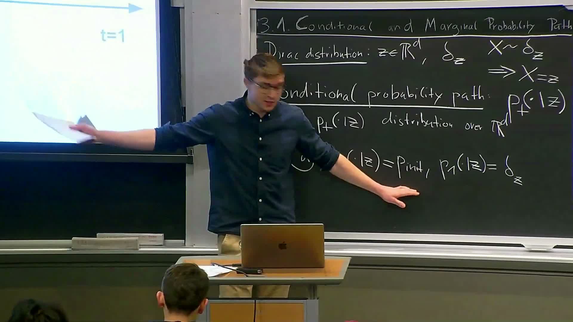
A probability path is a time-indexed family of probability distributions that interpolates between a simple initial distribution at t=0 and a target concentrated at a single data point at t=1.
-
The conditional probability path for a fixed data point z is written **p_t(x z)** and satisfies: -
**p_0(x z) = p_init(x)** (initial simple law) -
p_1(x|z) = δ_z (point mass at z)
-
- Canonical example — Gaussian interpolation (the “Gaussian path”):
p_t(x|z) = N(x; α(t) z, β(t) I)
where α(0)=0, α(1)=1 and β(0)=1, β(1)=0, so means and variances move from noise to the fixed data point.
This conditional construction provides a skeleton of intermediate distributions used to derive per-data-point vector fields and scores.
Marginal probability path and its density formula
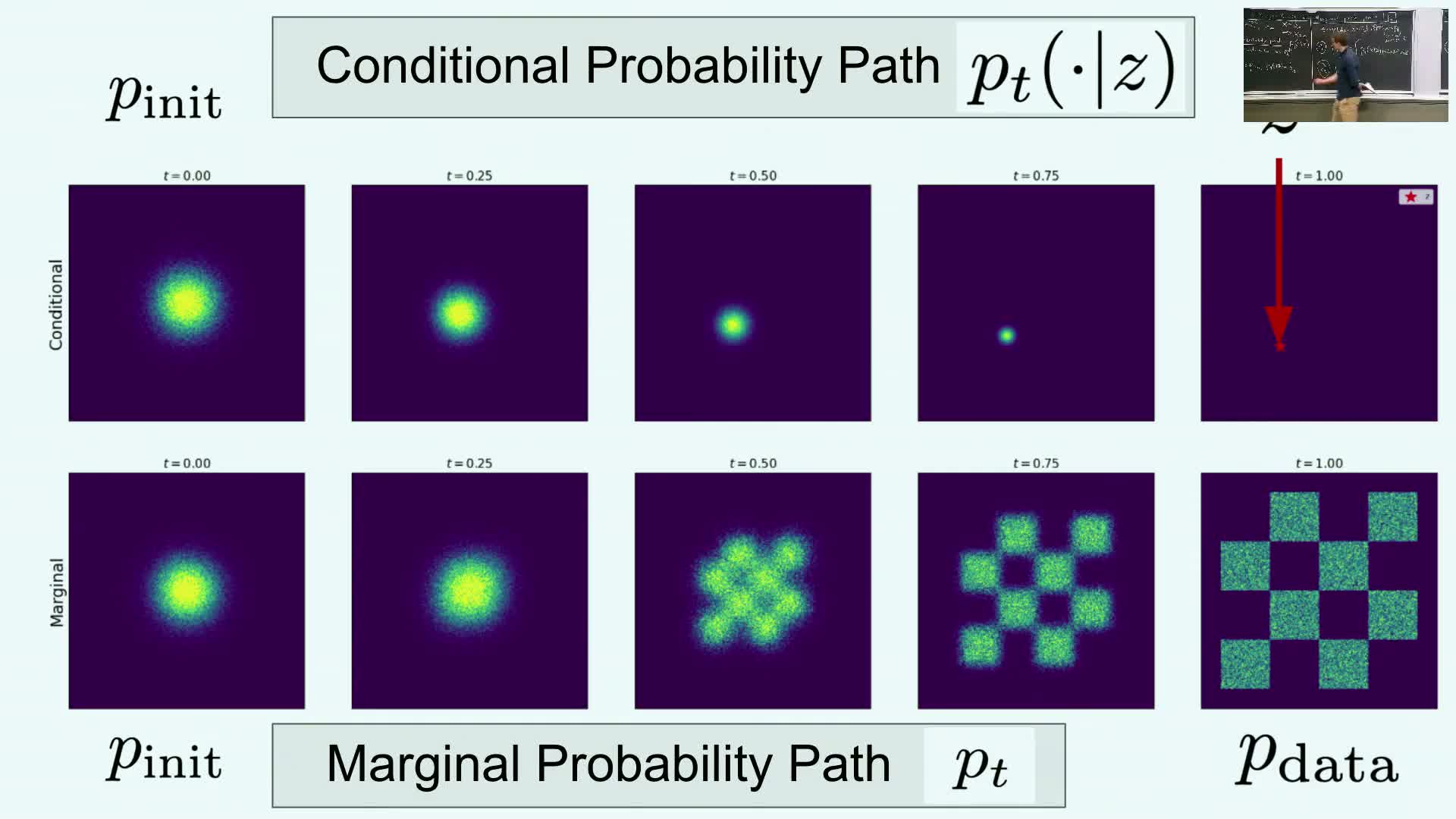
The marginal probability path is obtained by making the terminal data point z random under the data distribution and marginalizing it out:
p_t(x) = ∫ p_t(x|z) p_data(z) dz.
- This describes how the entire dataset’s distribution evolves over time.
- Boundary conditions are preserved:
- p_0(x) = p_init(x) (sampling at t=0 ignores z)
-
p_1(x) = p_data(x) (the path collapses to the data distribution at t=1)
The marginal density formula above gives an explicit expression for the marginal likelihood at any time t and is essential for later derivations of scores and marginal vector fields.
Conditional vector field and ODE construction per data point

A conditional vector field u_t(x; z) is a time-dependent vector field for a fixed data point z that defines an ODE dx/dt = u_t(x; z) whose solution X_t, initialized from p_init, has marginals p_t(·|z) at all times.
-
Defining requirement: when trajectories are simulated under u_t(x; z) starting from x_0 ~ p_init, the law of X_t equals **p_t(x z)** for every t.
- In practice, explicit formulas for u_t exist for common conditional paths. For the Gaussian conditional path, u_t(x; z) reduces to a simple affine combination of z and x with coefficients determined by α, β and their time derivatives (involving α̇ and β̇).
Constructing these per-data-point ODEs provides the building blocks for obtaining marginal dynamics by later marginalization.
Marginal vector field and the marginalization trick
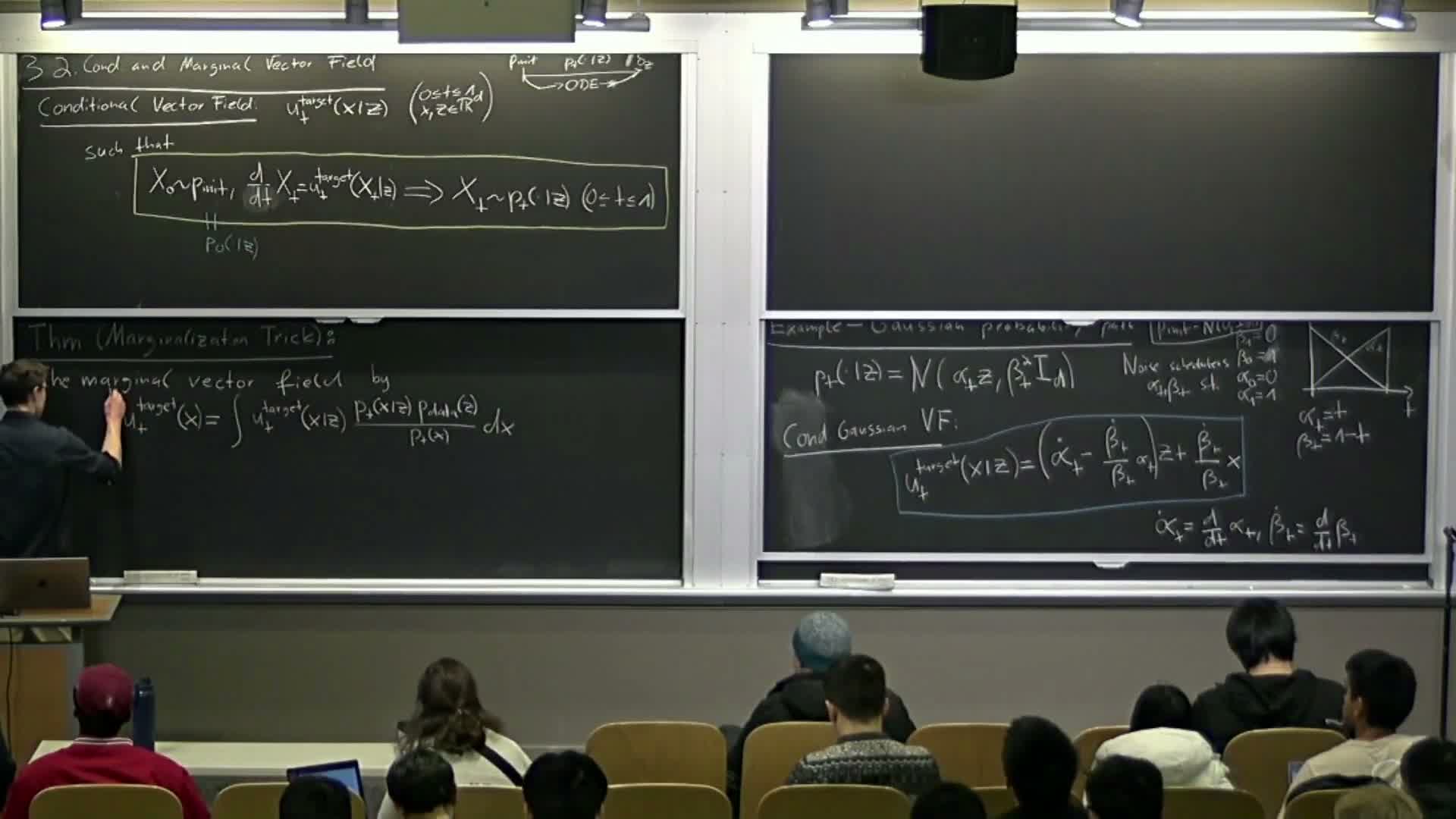
The marginalization trick defines a marginal vector field v_t(x) so that simulating dx/dt = v_t(x) produces trajectories whose marginals are the marginal probability path p_t(x).
- The marginal vector field is a posterior-weighted average of conditional vector fields:
v_t(x) = ∫ u_t(x; z) p_t(z|x) dz
equivalently
v_t(x) = (1 / p_t(x)) ∫ u_t(x; z) p_t(x|z) p_data(z) dz.
- Intuition: given a location x at time t, v_t(x) is the conditional expectation of the per-data-point drift under the posterior over which data point z could have produced x.
This formula converts per-data-point solutions into a single deterministic vector field that maps the initial noise distribution to the full data distribution when integrated.
Continuity equation and its role in proving marginalization
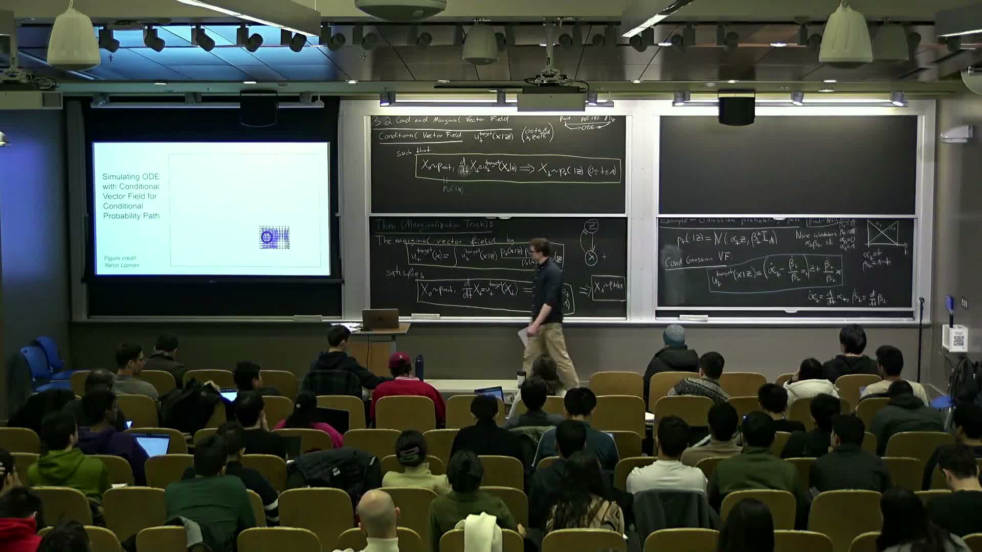
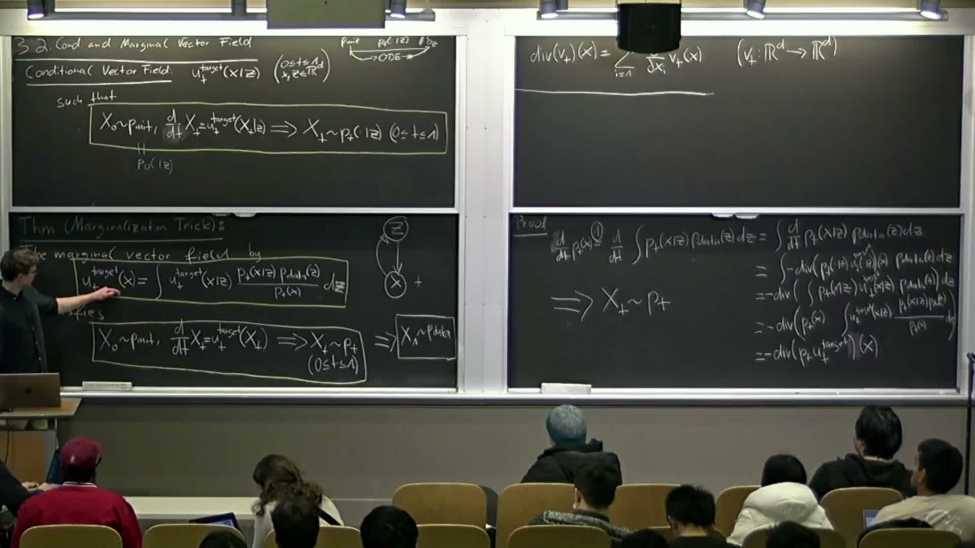
The continuity equation (aka the transport equation) links a vector field and a time-varying density:
∂_t p_t(x) = −∇·(p_t(x) v_t(x)), where ∇· denotes divergence.
- This equation is necessary and sufficient to ensure that the time evolution of the density under the deterministic flow induced by v_t matches the family {p_t}.
- Divergence is the net outflow/inflow operator; verifying the continuity equation for the marginal v_t defined by the posterior-weighted average of u_t(x; z) proves that integrating the marginal vector field yields the marginal probability path.
The continuity equation is the analytic bridge converting local conditional dynamics into a global marginal dynamics statement.
Proof sketch: deriving the marginal continuity equation from conditional dynamics
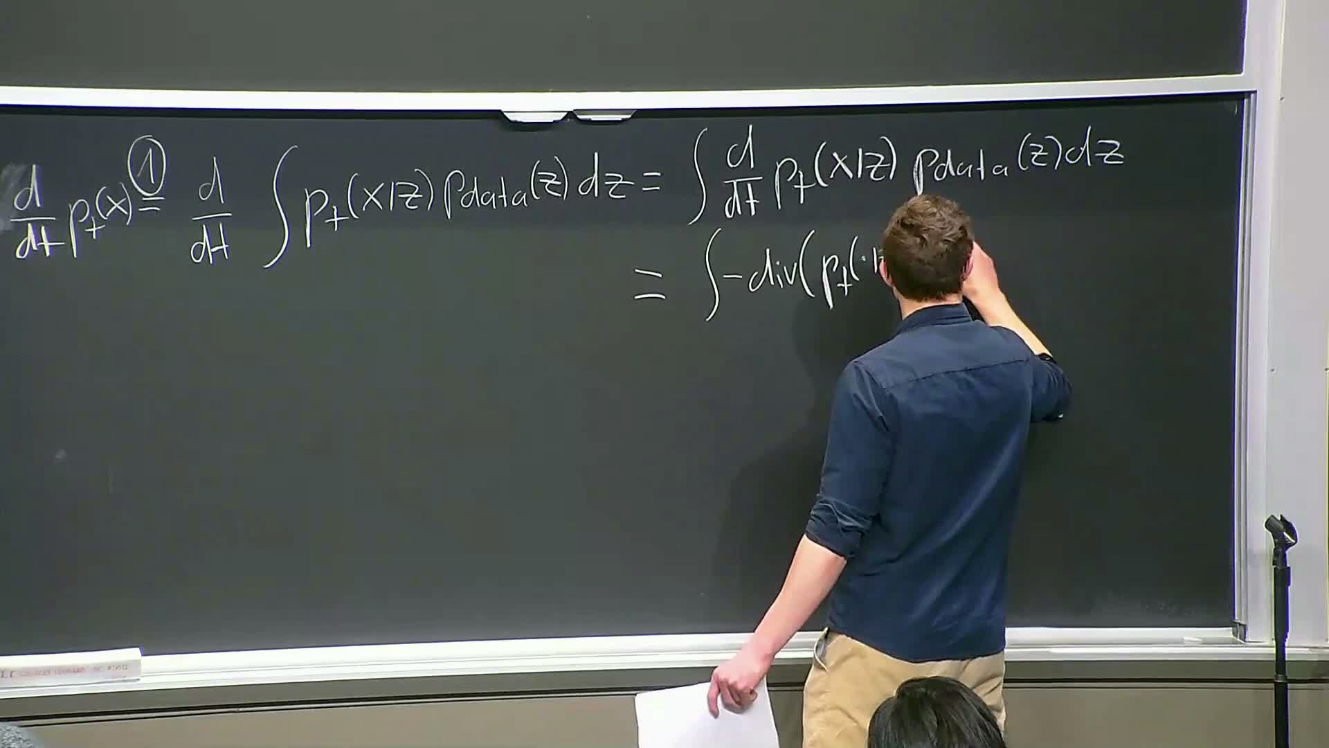
Proof sketch to verify the continuity equation for the marginal field:
-
Start from the marginal density **p_t(x) = ∫ p_t(x z) p_data(z) dz**.
- Under regularity assumptions, interchange differentiation and integration (Leibniz rule): differentiate under the integral sign.
-
Substitute the conditional continuity equation **∂_t p_t(x z) = −∇·(p_t(x z) u_t(x; z))**.
- Pull divergence outside the integral and algebraically multiply/divide by p_t(x) to identify the posterior-weighted average.
- Conclude ∂_t p_t(x) = −∇·(p_t(x) v_t(x)), i.e., the marginal continuity equation holds for v_t(x) defined as the posterior-weighted conditional drift.
This argument uses basic calculus identities (Leibniz rule, linearity of divergence) and the definition of v_t(x); it yields the sufficient condition that evolving with v_t maps p_0 to p_1 through the marginal path.
Visualization and intuition for flows mapping noise to data
Visual intuition and examples:
- Visualizations show conditional contour families and conditional vector fields that push mass from a noise distribution to a single data point z.
- Marginalization across data points produces a family of trajectories that convert noise into the full data distribution.
-
Key intuition: design u_t(x; z) per data point so the conditional law is **p_t(· z)**, then average appropriately to obtain a global deterministic flow that maps p_init to p_data.
These visual examples make concrete how local, z-parameterized flows align with global sampling behavior and illustrate that the analytic constructions can produce realistic samples (images, protein conformations, videos) when implemented at scale.
Score functions: conditional and marginal definitions and relation
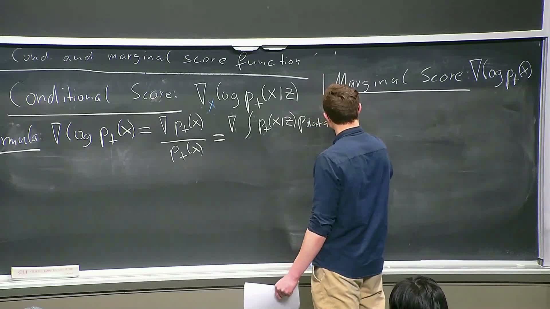
The score function is the gradient of the log-density with respect to x:
-
Conditional score: **s_t(x; z) = ∇_x log p_t(x z)**.
-
Marginal score: s_t(x) = ∇_x log p_t(x).
| The marginal score admits a posterior-weighted identity: **s_t(x) = ∫ s_t(x; z) p_t(z | x) dz**, obtained by differentiating **p_t(x) = ∫ p_t(x | z) p_data(z) dz** and applying the chain rule. |
Concrete Gaussian example: for the Gaussian conditional path, s_t(x; z) = −(x − α(t) z) / β(t), giving a simple closed-form conditional score. Score functions are central when converting deterministic flows to stochastic dynamics and when defining tractable training losses.
SDE extension (score correction) and the extension trick
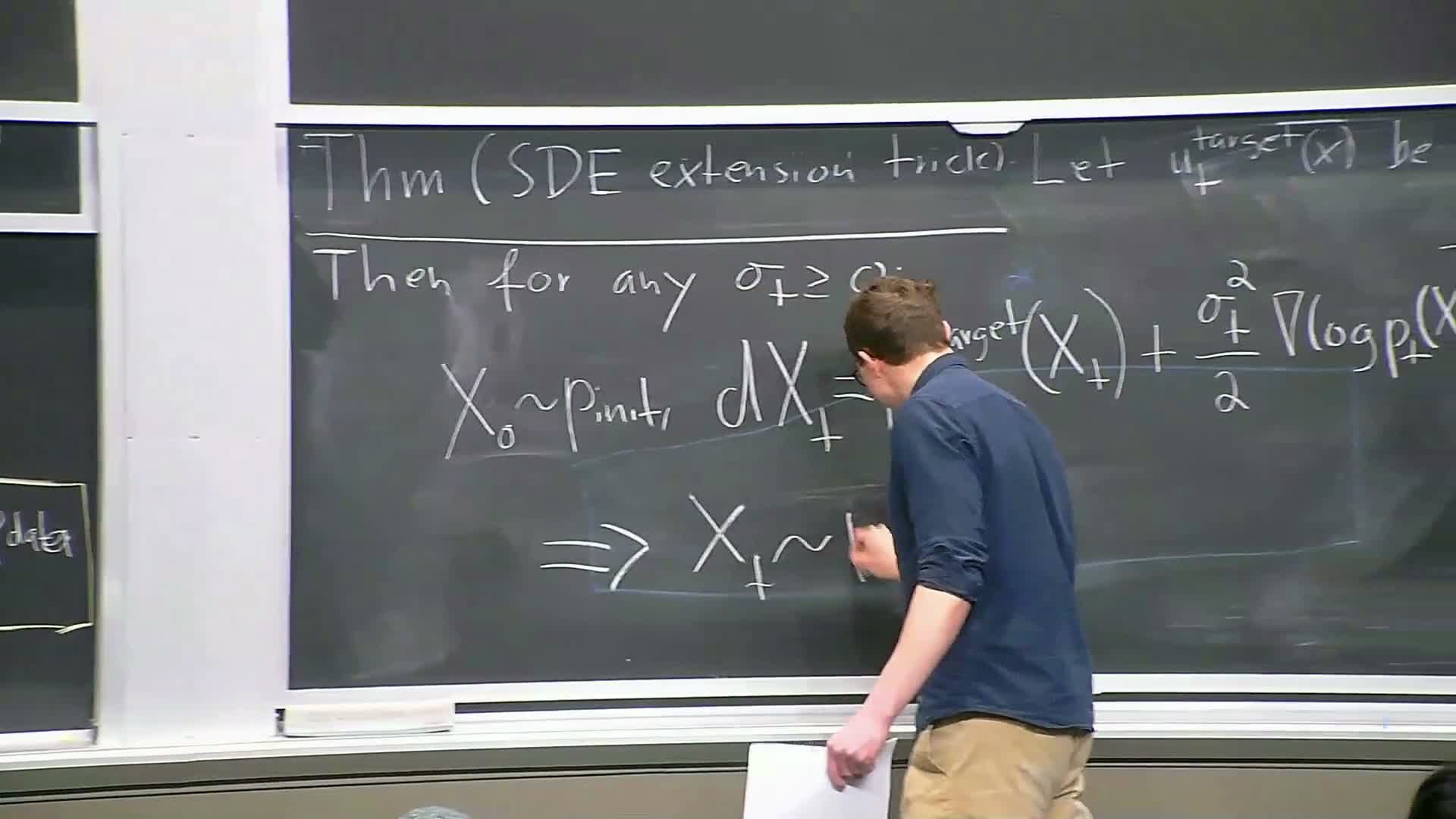
The extension trick generalizes deterministic marginal flows to SDEs by adding a diffusion term and a compensating drift correction involving the marginal score.
- For an arbitrary scalar diffusion coefficient σ(t), the SDE
dX_t = [ v_t(X_t) + (1/2) σ(t)^2 s_t(X_t) ] dt + σ(t) dW_t
(with W_t a standard Wiener process) yields marginal laws equal to p_t(·) provided v_t is the marginal vector field and s_t is the marginal score.
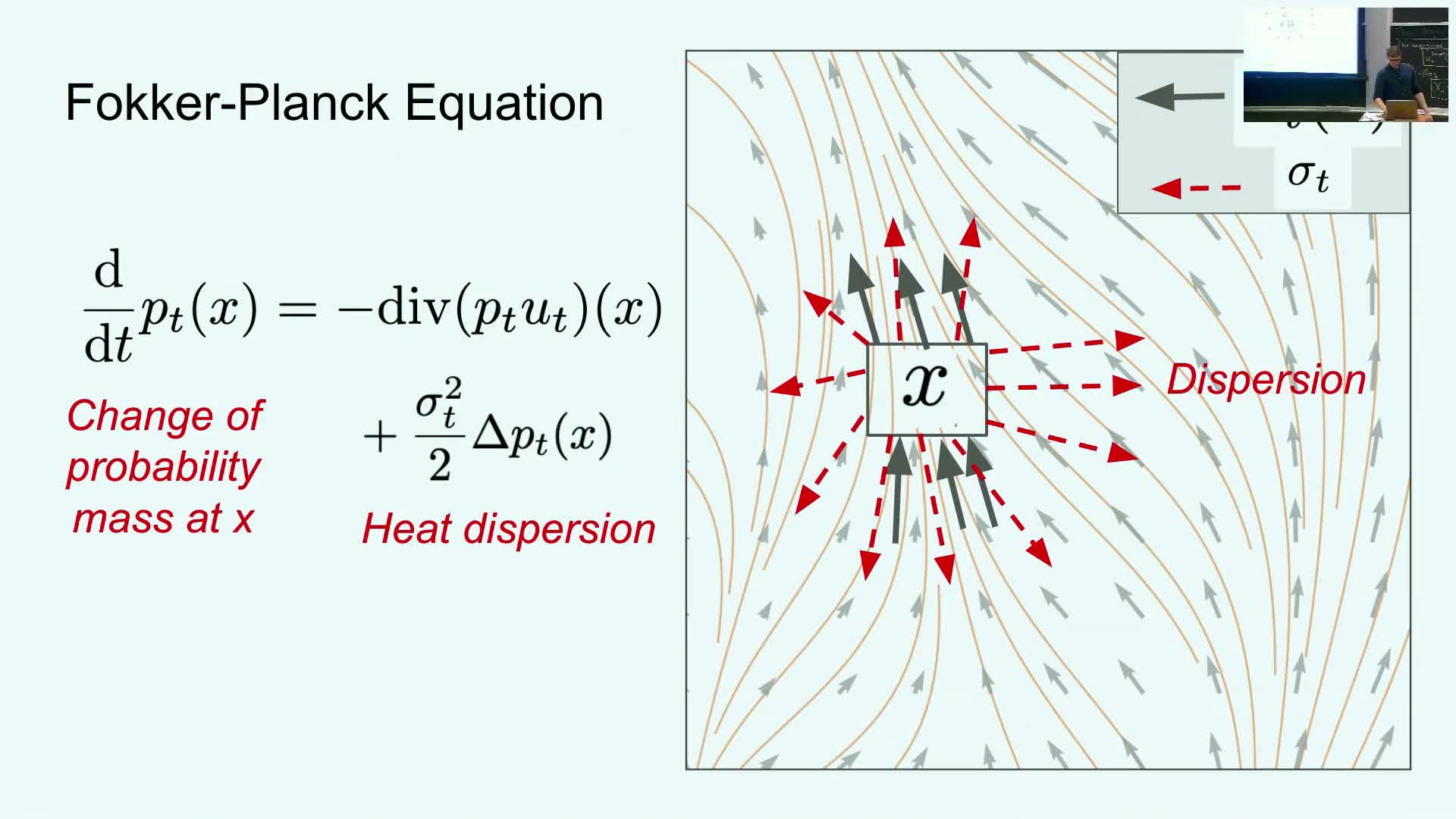
- The extra term accounts for the heat-like dispersion introduced by the injected noise.
- Consequence: many stochastic samplers (different σ schedules) share the same marginal path when the drift includes the appropriate score-based correction, giving a family of sampling dynamics that all map the initial distribution to the data distribution.
Practical implications, training target and course wrap-up
Practical goal and training perspective:
- The aim is to approximate one of the mathematical objects (typically the marginal vector field v_t or the marginal score s_t) with a neural network, then sample by integrating the corresponding ODE or SDE.
- Training reduces to deriving a loss that supervises the network to match conditional targets and, via marginalization identities, the marginal targets (e.g., score-matching objectives).
- The technically hardest step is deriving explicit formulas and identities for the six objects (conditional/marginal path, vector field, score). Once those are in hand, simple training losses allow efficient approximation without explicitly computing posterior integrals.
Implementation notes:
- The implementation/lab work focuses on the flow part (learning or approximating v_t and integrating the ODE).
- The score-related terms are a present-day extension used to inject noise when desired (enabling SDE samplers and certain training objectives).
The lecture closes by listing the six canonical formulas and preparing to present practical training losses (e.g., score-matching) in the next class.
Enjoy Reading This Article?
Here are some more articles you might like to read next: