MIT 6.S184 - Lecture 3 - Training Flow and Diffusion Models
- Overview of flows and diffusion models
- Conditional and marginal probability paths and associated vector/score fields
- Training objective: learn the marginal vector field with a neural network
- Flow matching loss definition and sampling protocol
- Intractability of direct marginal loss and the conditional surrogate
- Equivalence theorem: marginal and conditional losses differ by a theta-independent constant
- Practical flow-matching training algorithm
- Choice of time sampling and probability path
- Derivation for Gaussian conditional paths: reparameterization to noise
- ConPath (linear interpolation) yields a simple velocity prediction objective
- Intuition and empirical notes on path choice and application
- Quadratic identity proof sketch for equivalence of marginal and conditional losses
- Sampling from a trained flow and extension to diffusion models
- Score matching and denoising-score matching as the tractable surrogate
- Gaussian conditional path yields a denoising objective that predicts noise
- Numerical considerations and loss reparameterization for small noise levels
- Relationship between vector-field and score parameterizations and literature context
Overview of flows and diffusion models

Generative flows and diffusion models both construct complex data distributions by transforming a simple initial distribution through time-indexed dynamics.
-
Flow models use deterministic dynamics defined by an ordinary differential equation (ODE) with a vector field. Sampling = integrate the ODE from the initial latent distribution to the final time and take the terminal state as the sample.
-
Diffusion models use stochastic dynamics defined by a stochastic differential equation (SDE) with a drift (vector field) term and a diffusion (noise) term scaled by a time-dependent coefficient. Sampling = simulate the SDE and read the terminal time point.
The core sampling objective for both families is identical in spirit: ensure the final time of the simulated trajectory yields samples from the data distribution.
Conditional and marginal probability paths and associated vector/score fields
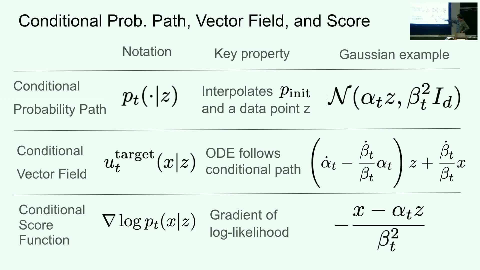
Conditional probability paths describe the interpolation between a fixed data point z and an initial distribution, producing:
-
a time-indexed conditional density **p(x_t z)**, and
-
an associated conditional vector field whose ODE trajectories follow that conditional path.
-
The conditional score is ∇_x log p(x_t z), i.e., the gradient of the conditional log density with respect to the instantaneous state.
Marginal probability paths arise by marginalizing over the data distribution:
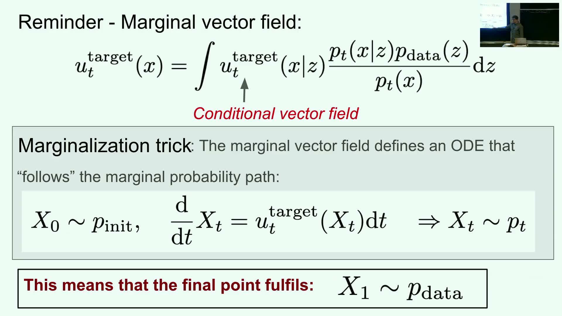
- they yield a marginal path p(x_t) that interpolates between p_init and p_data, and
-
an associated marginal vector field and marginal score that describe the dynamics of the marginal process.
- The marginal objects are the actual targets for generative modeling: simulating dynamics that follow the marginal path produces data samples at the final time.
-
Conditional and marginal objects are related by marginalization identities: marginal fields can be written as expectations or integrals over conditional fields weighted by **p(z x_t)** or equivalent ratios.
Training objective: learn the marginal vector field with a neural network
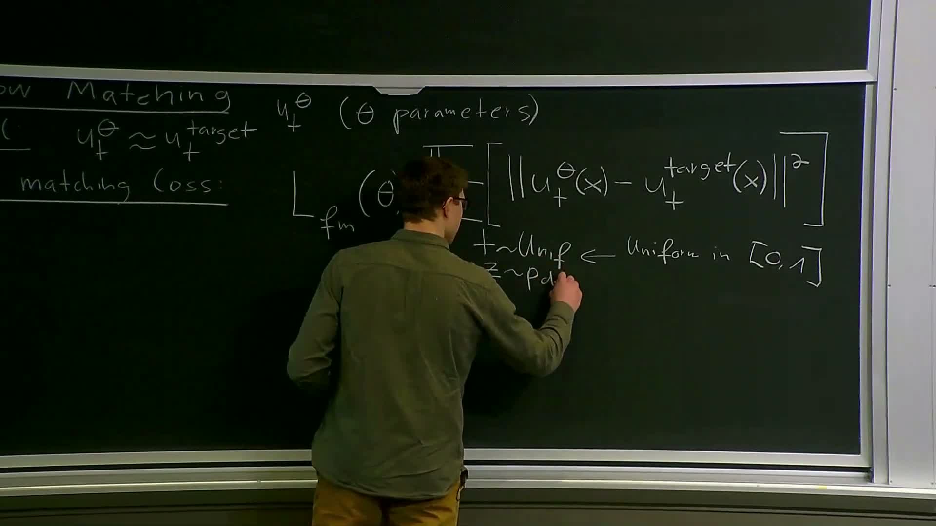
The training goal for flow models is to learn a time-dependent vector field u_t_theta(x) (a neural network) that approximates the marginal vector field v_t(x) which maps noise to data when integrated.
Formally:
- target: u_t_theta(x) ≈ v_t(x) for all t and x.
- training objective: minimize an expected mean-squared error between u_t_theta and the marginal target under an appropriate sampling of time and states.
Because the marginal target defines dynamics that transform the initial distribution into the data distribution, achieving this approximation suffices for generating realistic samples by ODE integration.
Flow matching loss definition and sampling protocol
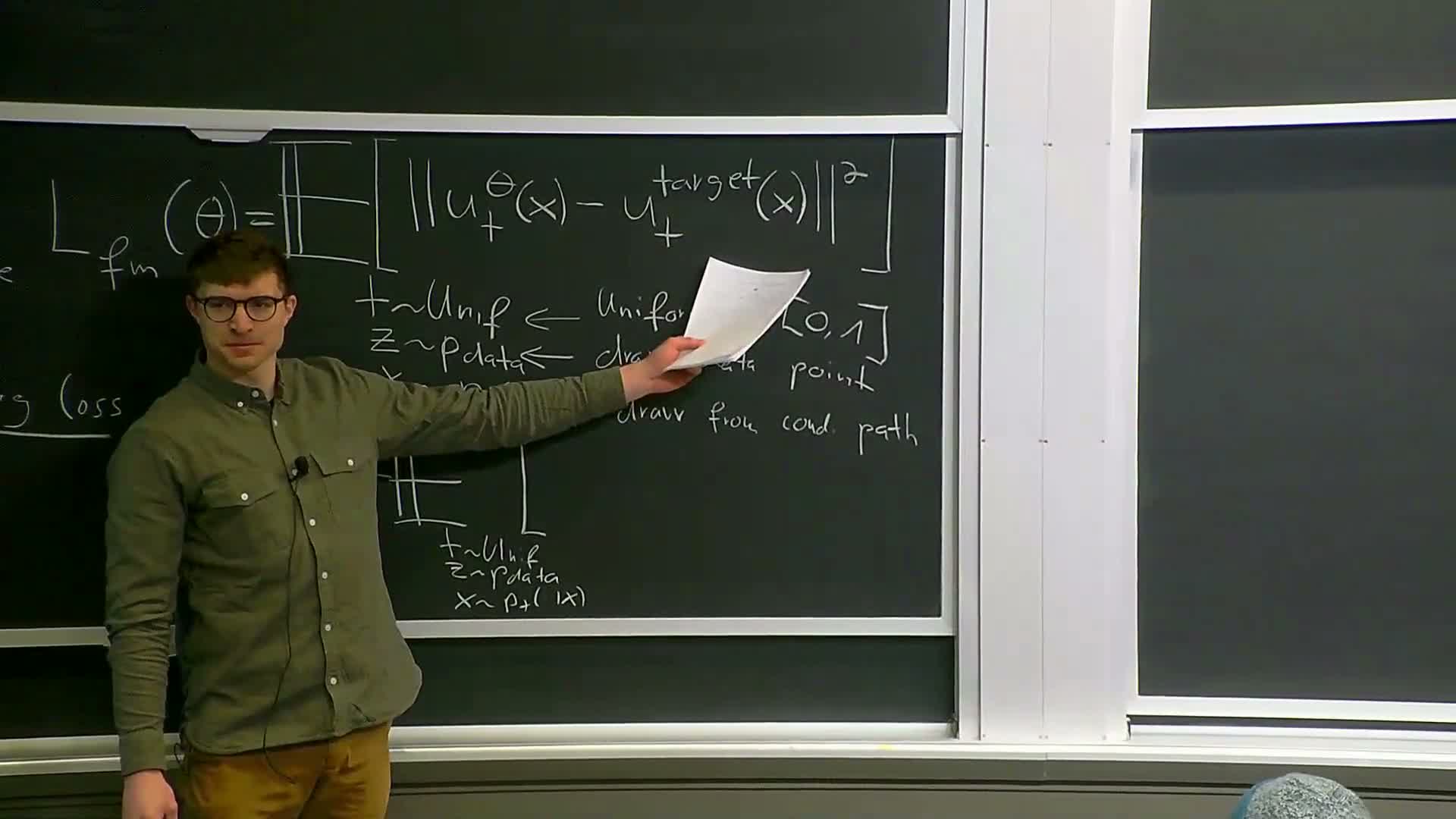
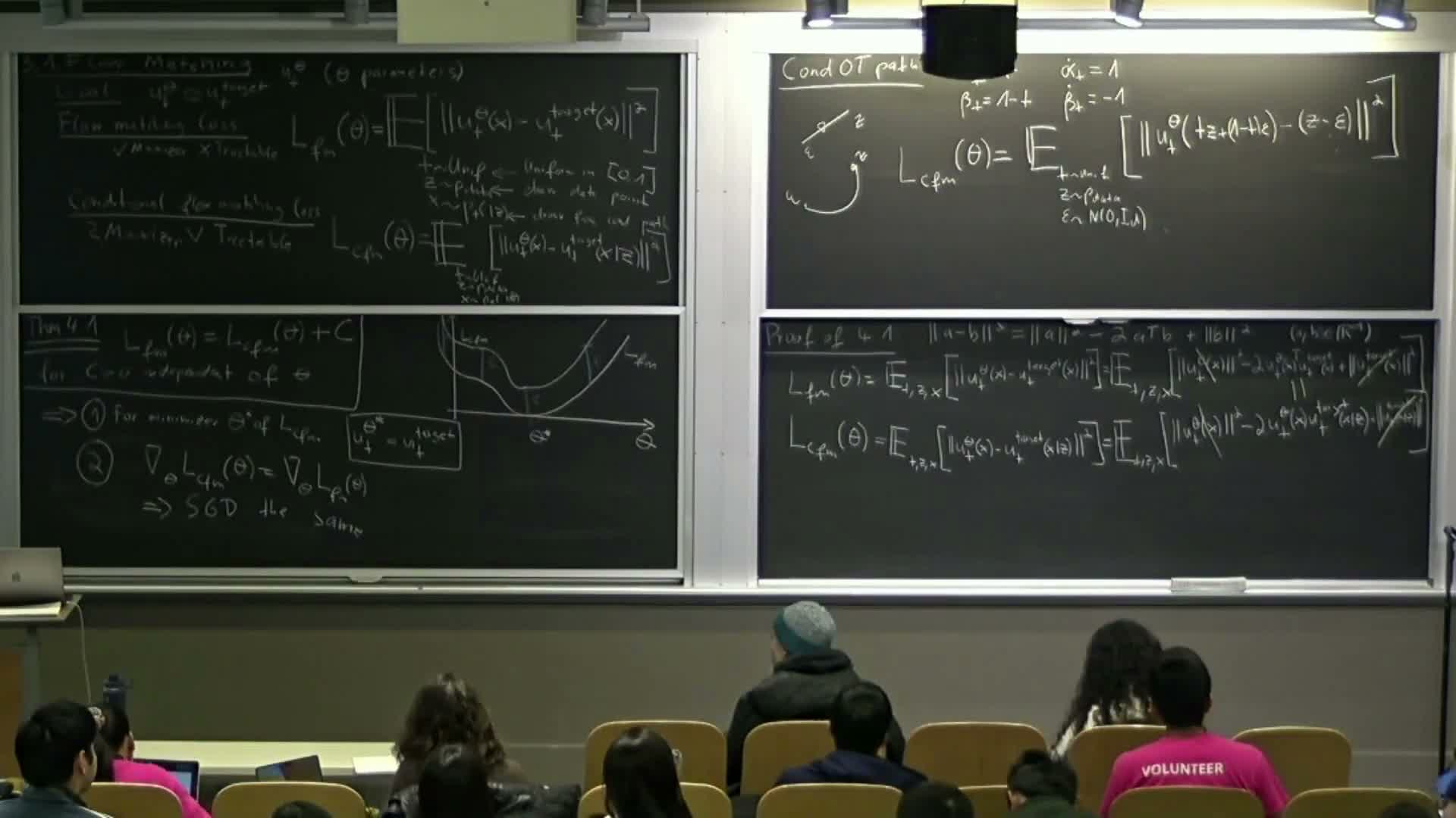
Flow matching training minimizes the expected squared error loss
-
L_flow = E_{t,x}[ ||u_t_theta(x) - v_t(x)||^2 ],
where the expectation is taken according to a sampling protocol for time t and state x.
A common practical sampling protocol:
- sample t uniformly in [0,1],
- draw a data point z from the dataset, and
-
draw x from the conditional distribution **p(x_t z)** induced by the chosen probability path.
- The loss is estimated by Monte Carlo (mini-batches).
- The network must accept both time t and spatial coordinates x as inputs and regress outputs to target vector values.
- While conceptually an MSE, the marginal form can be intractable due to nested integrals over the dataset.
Intractability of direct marginal loss and the conditional surrogate
The marginal flow-matching loss is intractable in general because the marginal target v_t(x) is an integral over all data points (a high-dimensional integral) that cannot be evaluated efficiently for each network evaluation.
- Direct evaluation would require summing/integrating contributions from the entire dataset for each sampled x and each optimization step — computationally infeasible for large datasets.
- Practical remedy: replace the marginal target in the loss with the conditional vector field, which is available in closed form for many designed probability paths.
This yields a conditional flow matching loss that is tractable and can be estimated using per-sample conditional draws.
Equivalence theorem: marginal and conditional losses differ by a theta-independent constant
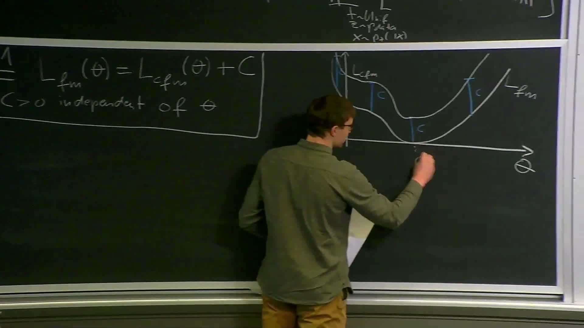
For the class of probability paths under consideration:
- the marginal flow matching loss equals the conditional flow matching loss plus a constant C that does not depend on the network parameters theta.
Consequences:
- Since C is independent of theta, the minimizer of the conditional loss coincides with the minimizer of the marginal loss.
- The parameter-space gradients of both objectives are identical.
Therefore, stochastic gradient descent on the tractable conditional loss follows the same training trajectory as if optimizing the intractable marginal loss — justifying the conditional loss as a faithful surrogate.
Practical flow-matching training algorithm
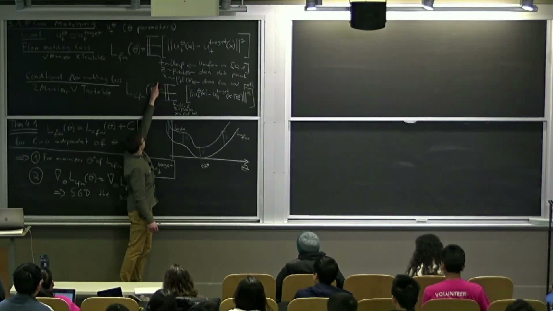
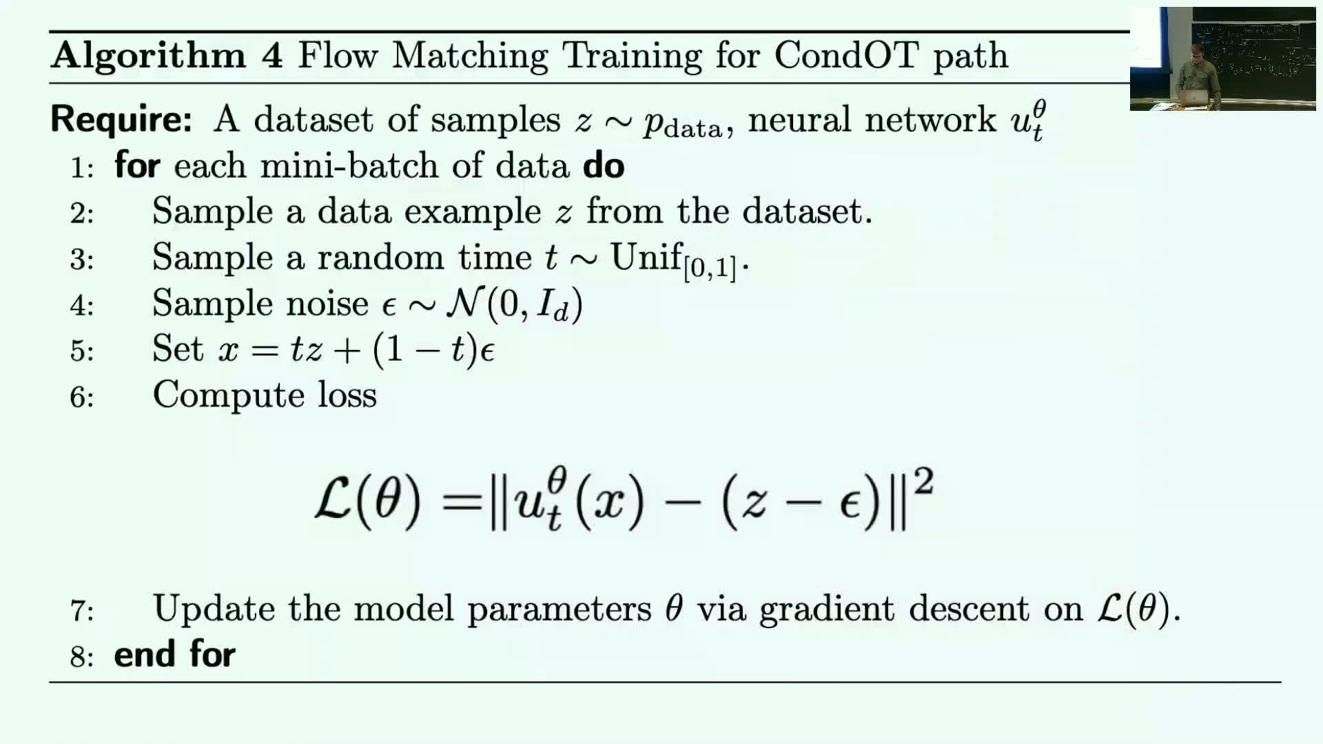
Flow-matching training procedure (iterative):
- sample a minibatch of data points z from the dataset,
- sample time t uniformly in [0,1],
-
sample x from the conditional distribution **p(x_t z)** induced by the chosen probability path,
-
compute the conditional flow matching loss u_t_theta(x) - v_t_conditional(x; z) ^2 using the analytic conditional v, and
- update theta by SGD or any optimizer.
- The neural network u_t_theta takes (t, x) as inputs and returns the predicted vector field at that state and time.
- Because many designed paths yield an analytic conditional vector field, training reduces to simple MSE regression with standard deep learning tooling and mini-batching.
Choice of time sampling and probability path

The sampling distribution over time t and the choice of conditional probability path are design hyperparameters that affect empirical performance but do not break the conditional-to-marginal equivalence.
-
Uniform time sampling is common because it treats all times equally.
- Alternative schemes (importance-weighted or non-uniform) may improve convergence by focusing updates on critical time regions.
- The conditional probability path is constrained only by boundary conditions (start at p_init, end at p_data).
- Different paths (e.g., straight-line interpolation, variance-preserving, variance-exploding) induce different conditional vector fields and numerical properties during simulation and training.
Derivation for Gaussian conditional paths: reparameterization to noise
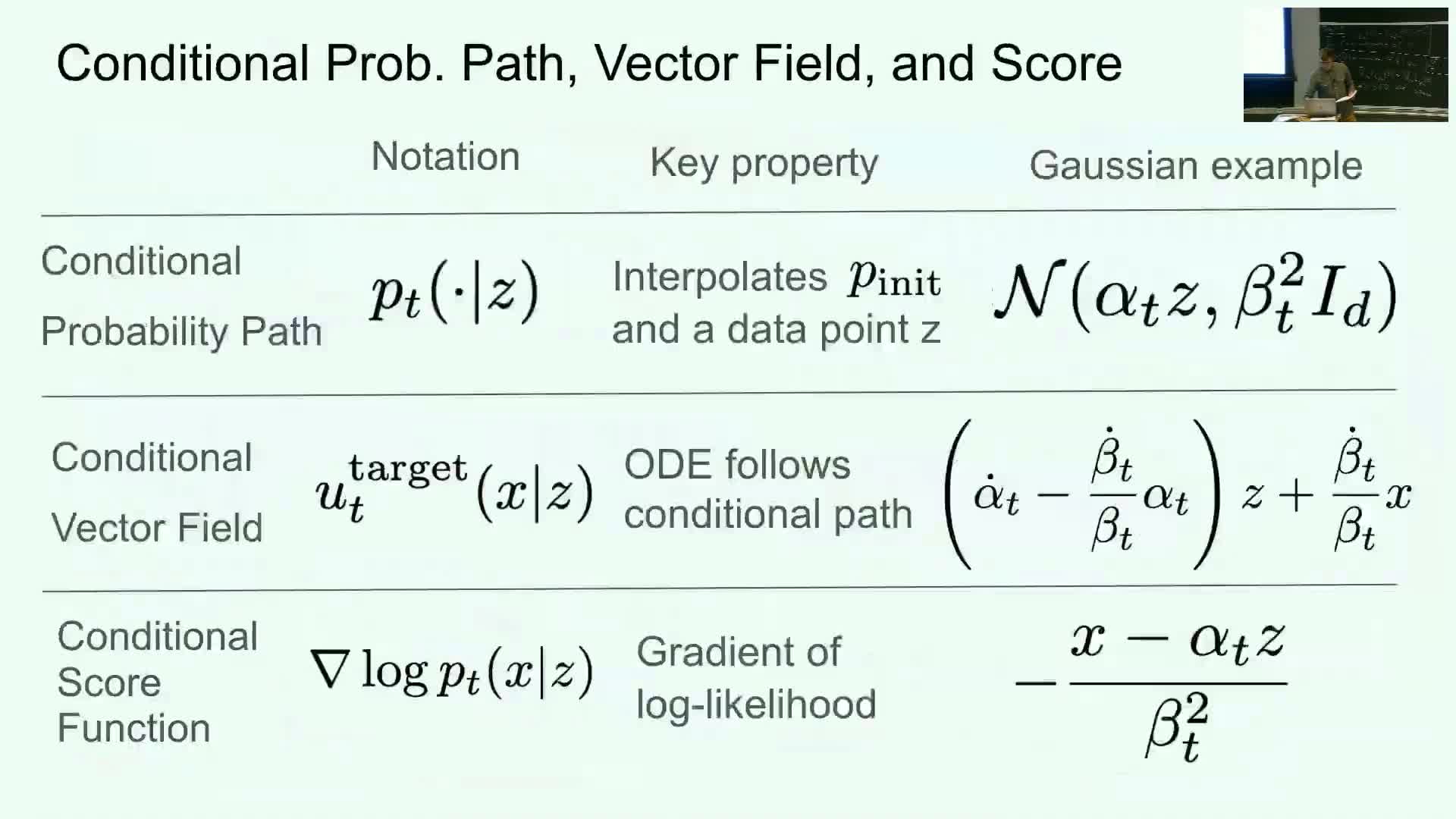
For Gaussian conditional probability paths with mean alpha_t z and variance beta_t, the conditional state can be reparameterized:
-
x = alpha_t z + beta_t epsilon, with epsilon ~ N(0,I).
Benefits:
- Sampling x becomes trivial: draw z from the dataset and standard Gaussian noise epsilon.
- This reparameterization allows substituting x into the conditional vector field formula and converts the expectation over x into an expectation over z and epsilon, yielding a tractable per-sample training target in closed form.
ConPath (linear interpolation) yields a simple velocity prediction objective

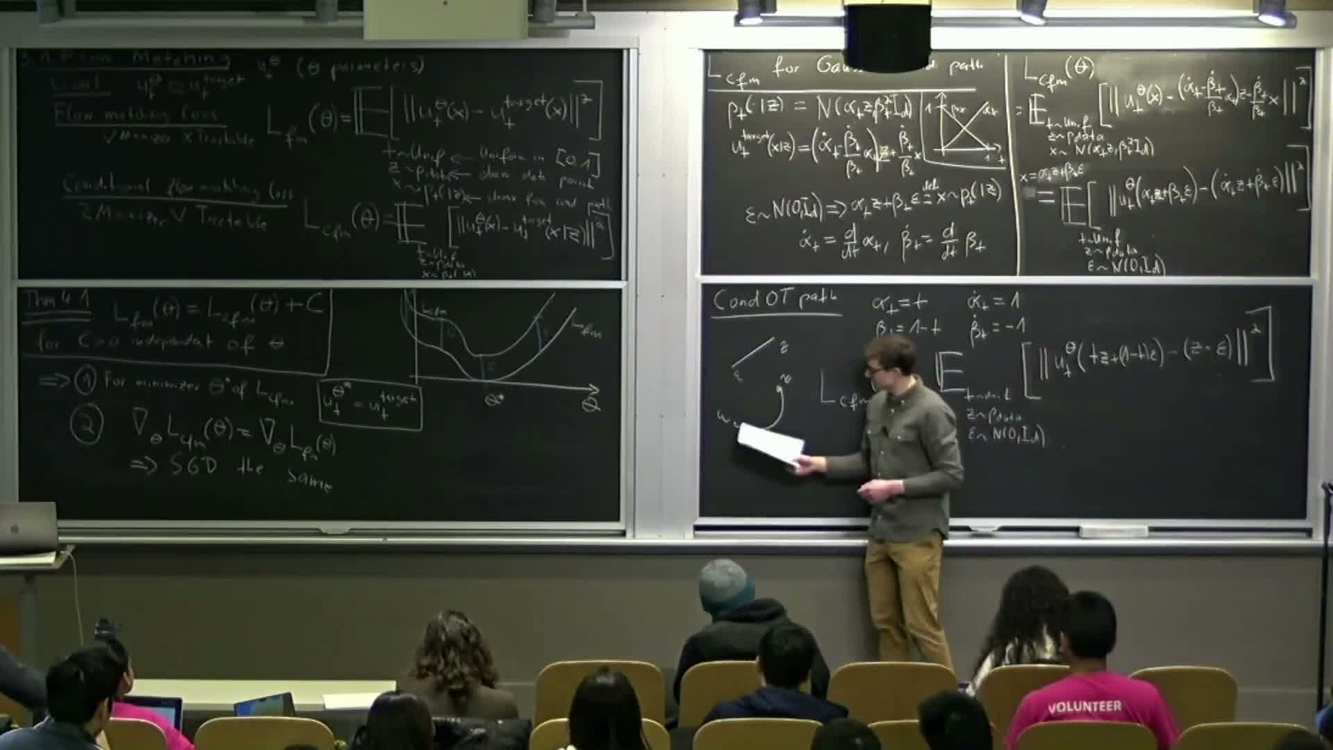
Choosing the linear interpolation path (alpha_t = t, beta_t = 1 - t) — often called the straight-line or conPath — yields a particularly simple conditional target:
- the network input is the convex combination x = t z + (1-t) epsilon, and
- the target vector often reduces to differences proportional to z - epsilon (up to scalar factors) in many constructions.
Simple training algorithm:
- sample z from the dataset,
- sample epsilon ~ N(0,I),
- sample t uniformly,
- form x = t z + (1-t) epsilon, input (t, x) to the network, and
- regress to the scaled displacement between data and noise.
Interpretation: the network learns instantaneous velocities along the straight-line path from noise to data — a basis for many practical implementations.
Intuition and empirical notes on path choice and application
The conditional-path velocity interpretation gives useful intuition about information and difficulty over time:
- At early times the state is dominated by noise → the network has limited information about z and predictions are harder.
- At late times the state approaches z → predictions become easier.
Empirical trade-offs:
- Different paths (straight-line, variance-preserving, variance-exploding) trade off numerical stability and integration error during sampling.
- Straight-line interpolation can reduce integration error, while other schedules may offer advantages in specific settings.
Many contemporary image and video diffusion systems use variants of these conditional training objectives and path choices, leveraging simple MSE regression within high-performance architectures.
Quadratic identity proof sketch for equivalence of marginal and conditional losses

The equivalence proof rests on a quadratic identity and linearity of expectation:
-
Start from the identity ** A - B ^2 = A ^2 + B ^2 - 2⟨A,B⟩** and apply it to both marginal and conditional losses to expand squared errors.
- Terms depending only on the model but not on theta cancel when comparing the two losses.
- The remaining cross term is linear in the data z, so its expectation commutes with marginalization over z; the cross-term expectations match.
After removing theta-independent constants and matching cross-term expectations, the two objectives differ only by a constant independent of theta, proving identical minimizers and gradient fields.
Sampling from a trained flow and extension to diffusion models
Once the marginal vector field has been learned to sufficient accuracy, the generative sampler is simply an ODE integrator that simulates:
- dx/dt = u_t_theta(x) from p_init to the final time, producing samples from p_data at the endpoint.
The same paradigm generalizes to stochastic dynamics:
-
Diffusion models require learning a marginal score function s_t(x) that converts an SDE into a sampling SDE or provides targets for reverse-time simulation.
- The training formalism mirrors flow matching: define a marginal score loss and a tractable conditional surrogate (the denoising objective), use an equivalence that preserves minimizers up to a constant, and train by MSE regression.
Score matching and denoising-score matching as the tractable surrogate

Score matching aims to learn parameters theta for s_t_theta(x) that approximate the marginal score ∇_x log p(x_t).
- Natural loss: expected squared error between s_t_theta and the marginal score.
-
The marginal loss is intractable for the same reasons as in flow matching, but a conditional denoising score (∇_x log p(x_t z)) is often analytically available and serves as a tractable surrogate.
A key theorem analogous to flow matching: the marginal score-matching loss equals the denoising surrogate up to a theta-independent constant, so minimizing the tractable denoising loss yields the correct marginal score in the limit of perfect optimization.
Gaussian conditional path yields a denoising objective that predicts noise
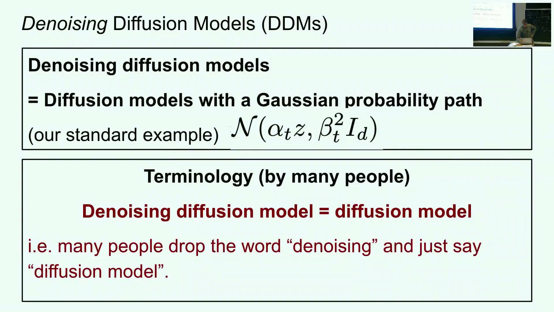
For Gaussian conditional paths with x = alpha_t z + beta_t epsilon, the denoising-score-matching target simplifies:
- predict the noise scaled by 1 / beta_t, or equivalently predict epsilon after appropriate reweighting.
Concrete training procedure:
- sample z and epsilon,
- form x = alpha_t z + beta_t epsilon,
- input (t, x) to the score network, and
- regress the network output to the appropriate scaled-noise term.
This is the canonical denoising objective used in many diffusion implementations — the method learns to predict the corruption noise that turned z into x.
Numerical considerations and loss reparameterization for small noise levels
When beta_t is small (times near the final data endpoint), the scaled score target (noise divided by beta_t) can have very large magnitude and variance, causing numerical instability and high-variance gradients.
Practical fixes:
- reparameterize the network to predict normalized noise (epsilon) directly (noise predictor), or
- scale the loss with beta_t-dependent weights to stabilize gradients.
These numerical techniques preserve the theoretical equivalence while improving training stability and are standard in diffusion literature.
Relationship between vector-field and score parameterizations and literature context
For the Gaussian (denoising) conditional path both the conditional vector field and the conditional score are affine combinations of z and x with known coefficients, which implies:
- algebraic convertibility between the vector-field parameterization and the score parameterization.
Consequences and context:
- For denoising diffusion models one can train in either parameterization and convert the learned mapping post-hoc; early influential systems used score-only training because conversion to vector fields was possible.
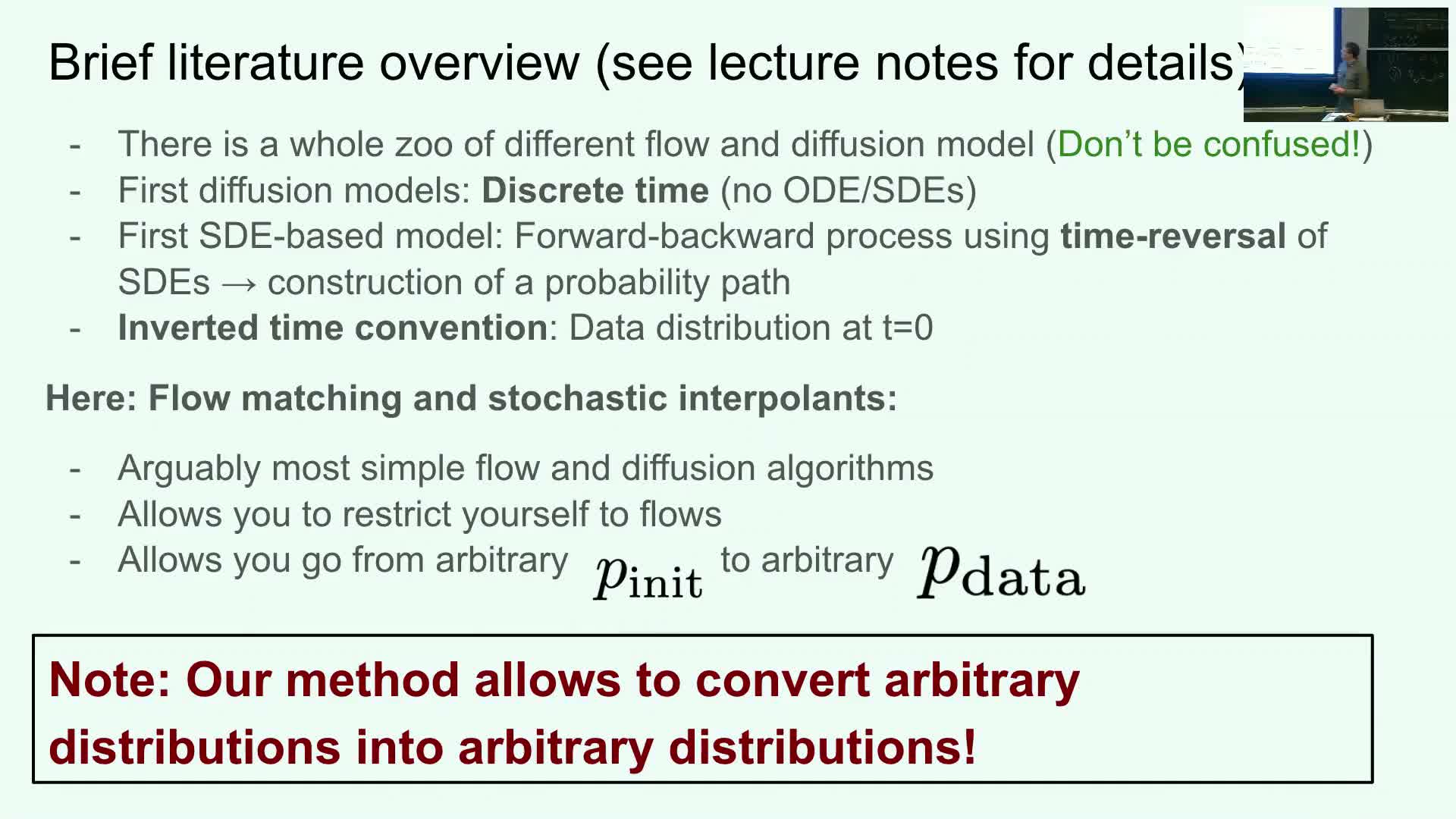
- The literature contains multiple equivalent formulations (discrete-time diffusion, time-reversed SDEs, stochastic interpolants, flow matching) that differ in conventions and numerical choices.
- Practical implementations select among these formulations based on ease of integration, numerical stability, and sampling efficiency.
Enjoy Reading This Article?
Here are some more articles you might like to read next: