MIT 6.S184 - Lecture 4 - Building an Image Generator
- Course introduction and scope
- Conditional versus unconditional generation and objectives recap
- Sampling dynamics and lecture agenda
- Guided generation notation and examples of conditioning variables
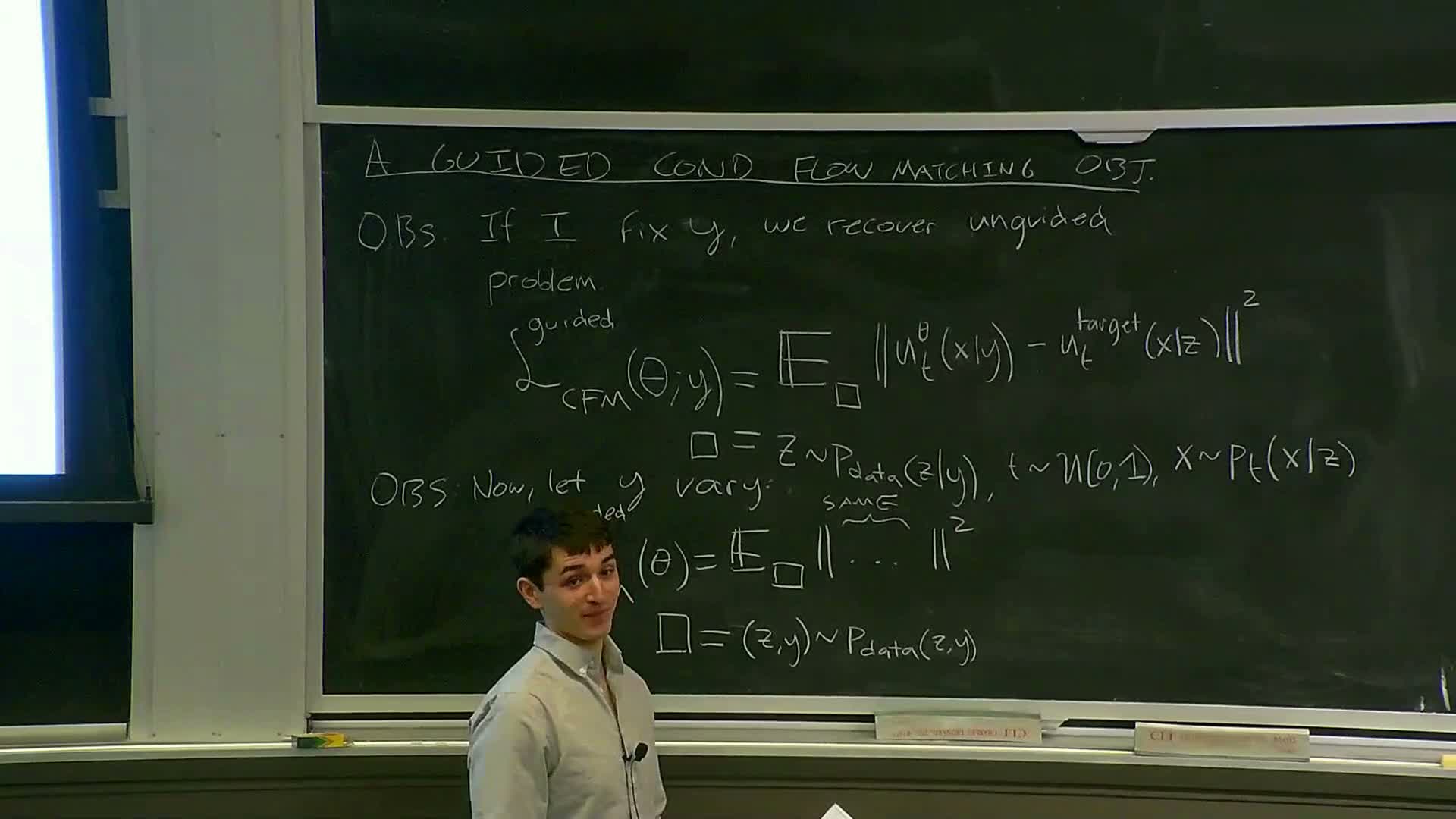
- Guided conditional flow matching objective: fixed y and amortization over y
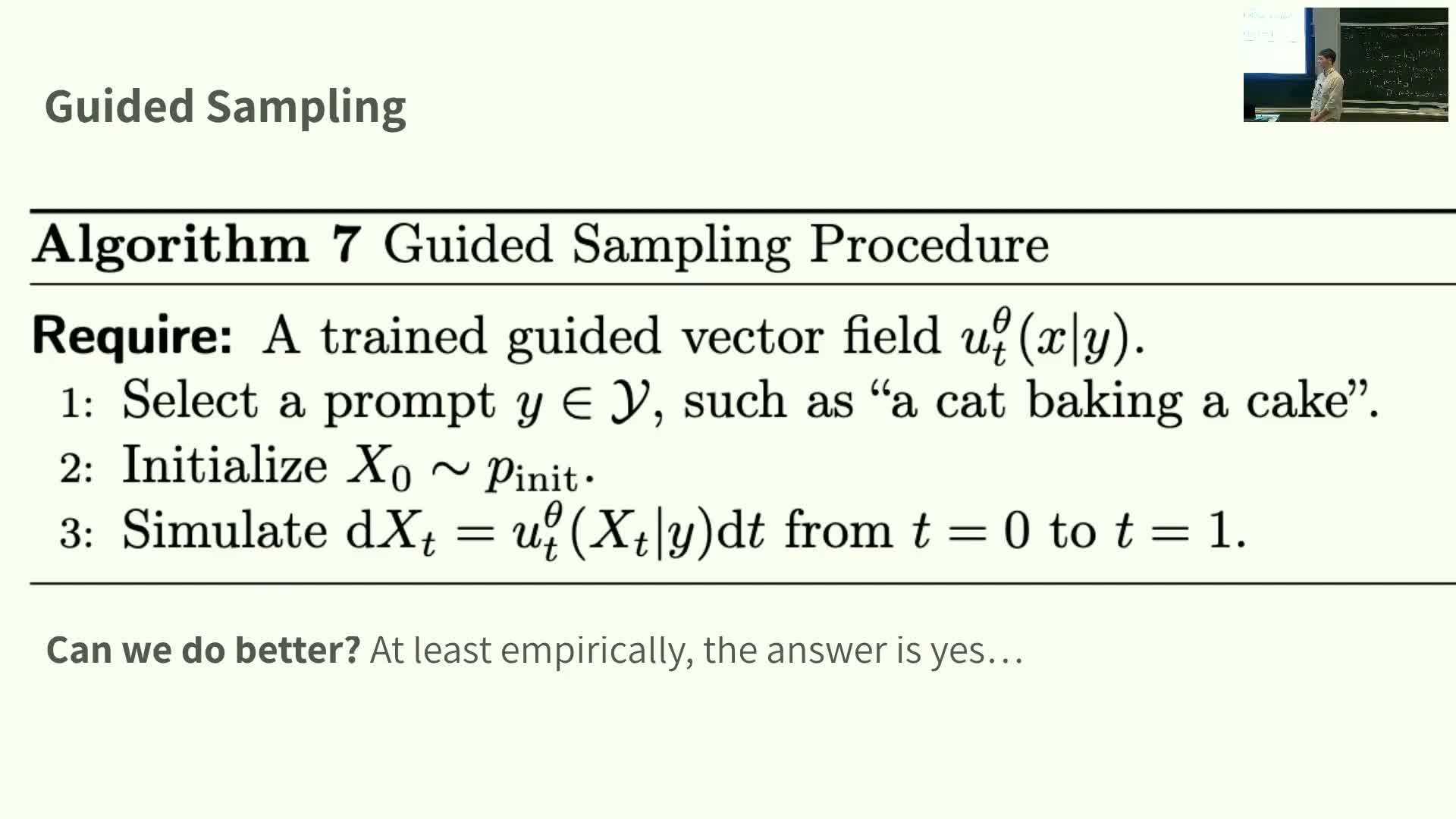
- Training and sampling with guided vector fields
- Introduction to classifier-free guidance and motivation
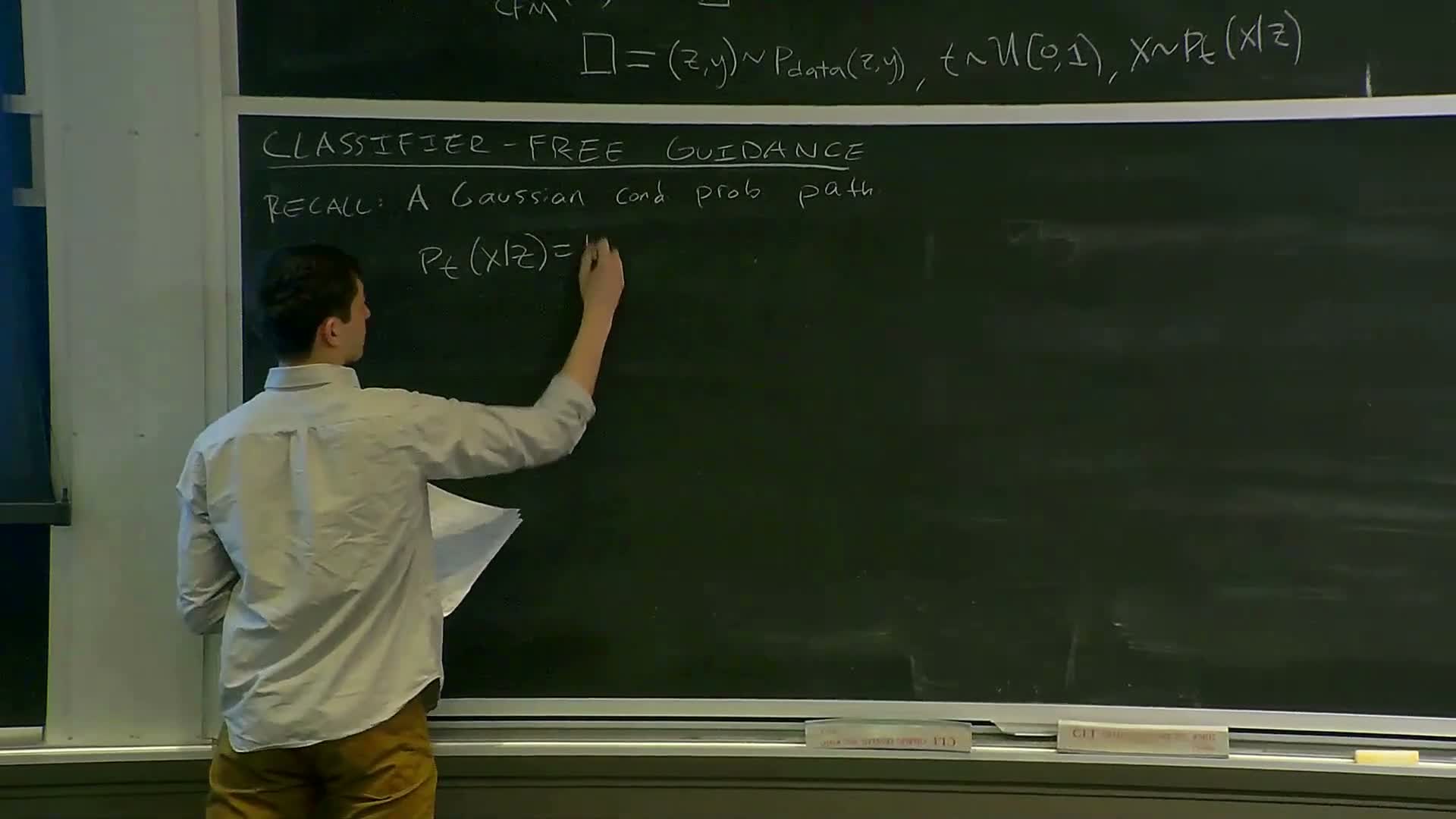
- Gaussian conditional probability paths and relation between vector fields and scores
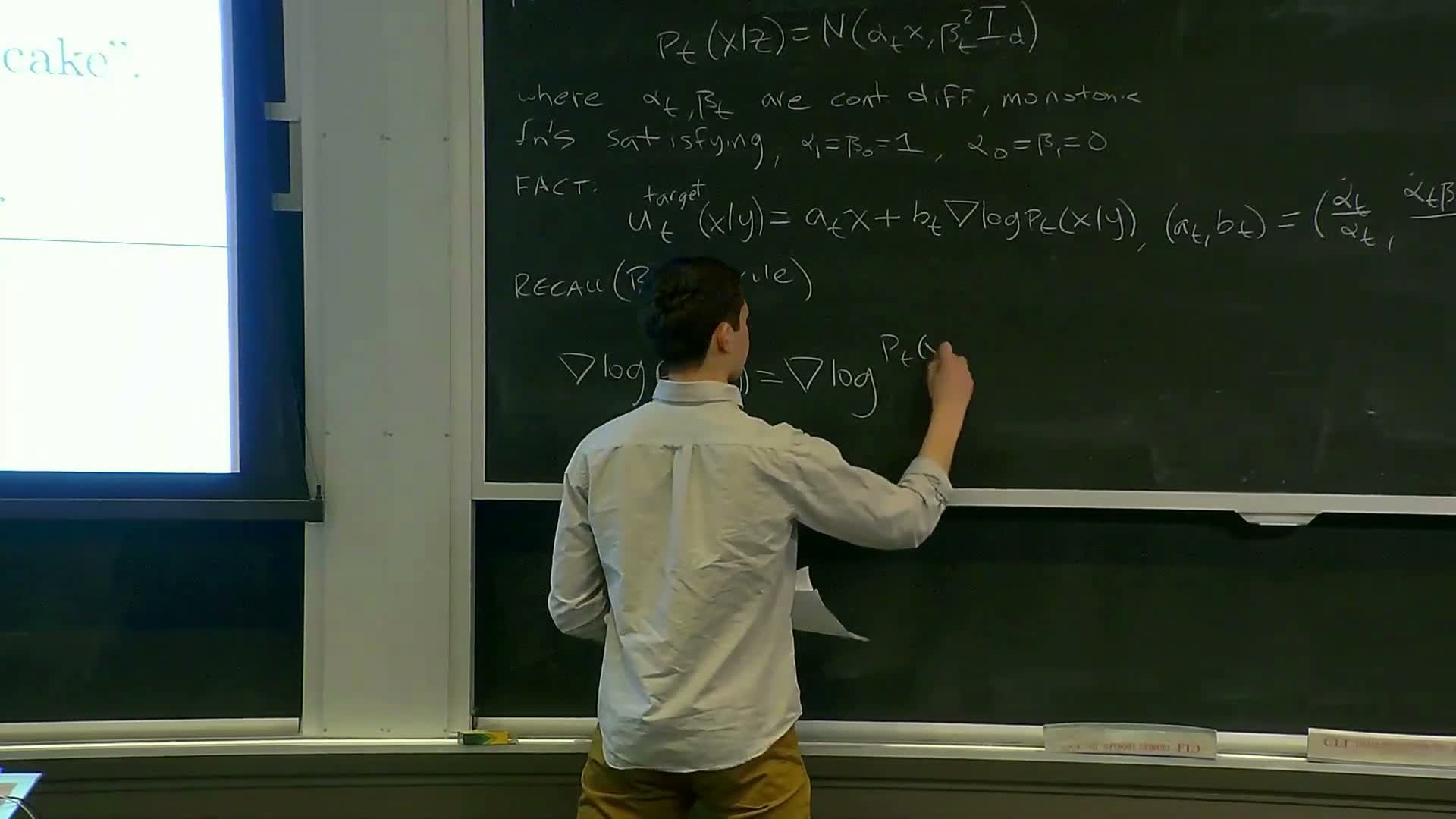
- Bayes decomposition of the guided score and identification of a classifier term
- Guidance scaling factor and constructing an amplified guided vector field
- Algebraic rearrangement to classifier-free guidance and single-model training with null token
- Practical sampling with CFG and empirical MNIST example
- Real-world CFG examples and discussion of classifier identity and effects
- Image data structure and why MLPs are insufficient for high-resolution images
- UNet architecture overview for diffusion/flow models
- Residual layer internals and conditioning injection in UNet
- Diffusion Transformer (patch-based attention)
- Latent-space modeling and the latent diffusion design pattern
- Stable Diffusion 3 case study and multimodal conditioning
- Course logistics and transition to guest lecture
- Guest lecture introduction: reward fine-tuning for flow and diffusion models
- Fine-tuning objective as KL-regularized optimization and SDE/flow connections
- Flow matching, SDE sampling equivalence, and the role of arbitrary noise schedules
- Stochastic optimal control interpretation of fine-tuning and necessity of memoryless noise schedules
- Agent method for solving the control problem and adjoint/agent matching
Course introduction and scope

This segment introduces the lecture objectives and places the session in course context.
- The lecture transitions from unconditional to conditional generation tasks, using image generation as the running example.
- Prior lectures developed training objectives such as conditional flow matching and denoising score matching; this session will focus primarily on flow models while noting analogous results for diffusion models.
- The practical goal is conditioning generative models on auxiliary information (e.g., text prompts or labels).
- The instructor stresses that scaling the parameterization is required for real-world image synthesis.
- This overview frames a theory-to-practice agenda and invites students to interrupt with questions as needed.
Conditional versus unconditional generation and objectives recap
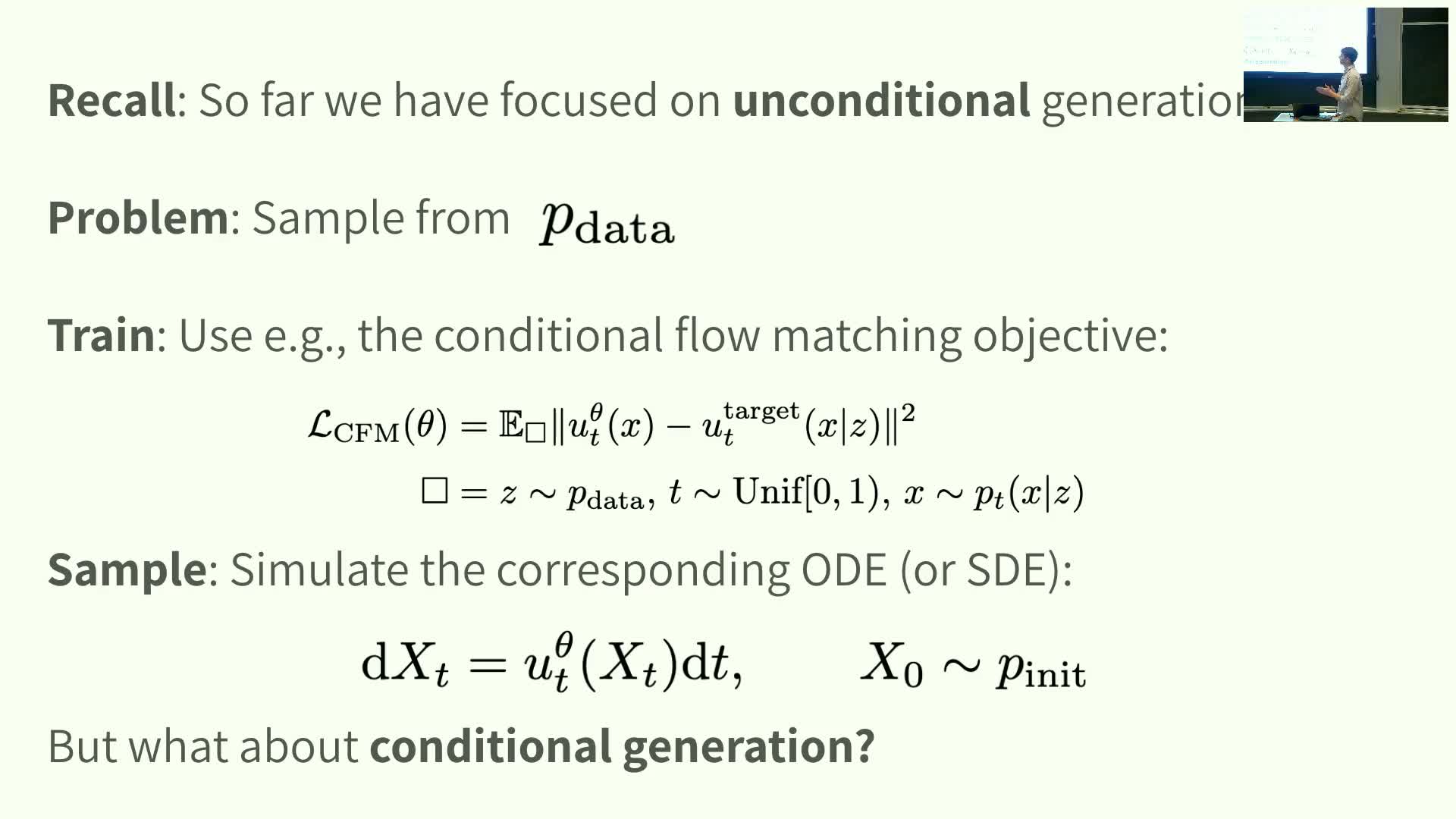
This segment defines the conditional generation problem and connects it to previously developed objectives.
-
Problem statement: sample from the data distribution conditioned on auxiliary information y, i.e., from **p_data(x y)**.
- Reiterated objectives:
-
Conditional flow matching for flow-based models.
-
Denoising score matching for diffusion/score-based models.
-
Conditional flow matching for flow-based models.
-
Technical mechanism (flow view): learn a conditional vector field **u_t^θ(x y)** by regressing it against a conditional target vector field.
- Integrating the learned field yields an ODE sampler that maps an initial noise distribution to the data manifold.
-
In the ideal case of perfect learning, this recovers **p_data(x y)** exactly.
- Integrating the learned field yields an ODE sampler that maps an initial noise distribution to the data manifold.
- Narrative choice: lecture focuses on flow models for clarity, with diffusion equivalents available in the notes.
- Takeaway: conditional objectives extend the unconditional training pipeline by conditioning all path distributions, vector fields, and regression targets on y.
Sampling dynamics and lecture agenda
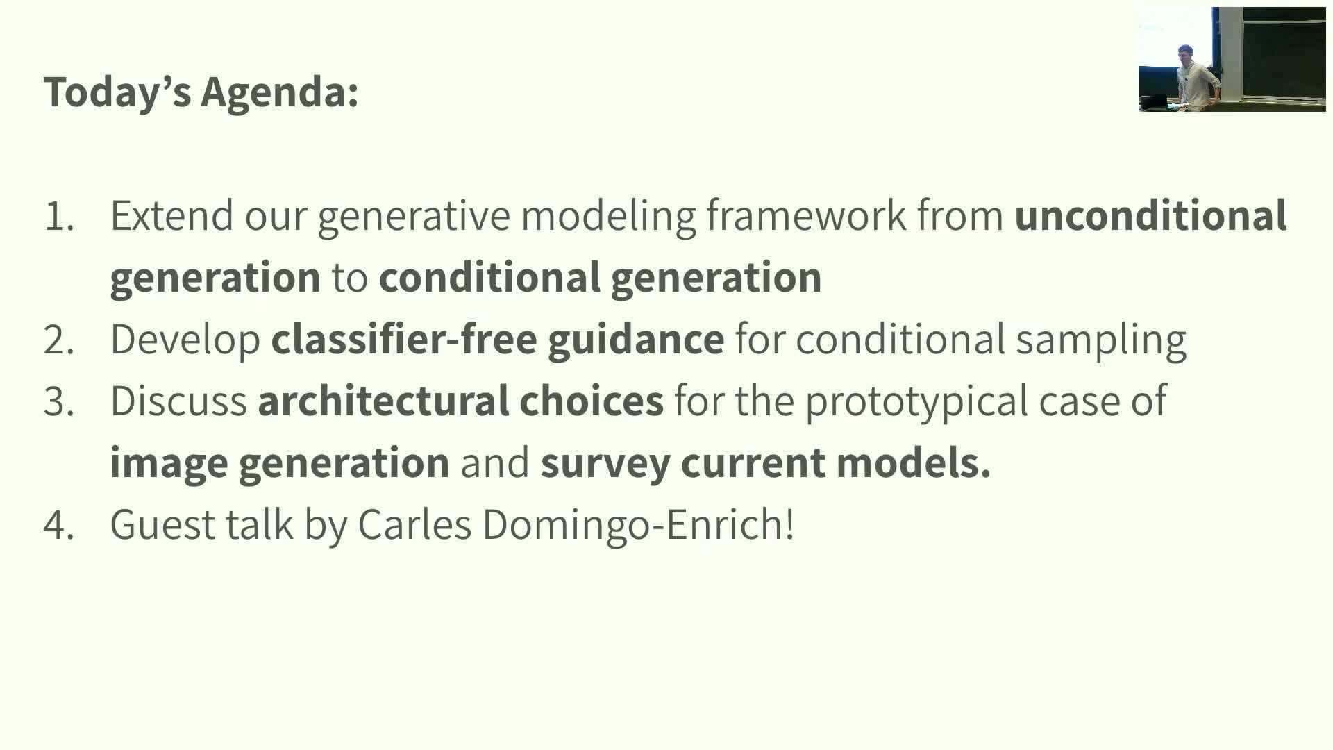
This segment summarizes sampling after training and outlines the lecture agenda.
- Sampling after training:
- Simulate the learned ODE (or the equivalent SDE when using scores) from the initial noise time z to t = 1.
-
Under perfect learning, samples from this simulation follow **p_data(x y)**.
- Simulate the learned ODE (or the equivalent SDE when using scores) from the initial noise time z to t = 1.
- Lecture plan:
- Extend unconditional generation methods to conditional settings.
- Present classifier-free guidance (CFG) for conditional sampling.
- Discuss architectural choices for image generation (UNets, diffusion Transformers, latent models).
- Survey modern models (including Stable Diffusion 3).
- Introduce a guest lecture on alignment / reward fine-tuning.
- Extend unconditional generation methods to conditional settings.
- Practical emphasis: moving from low-dimensional examples to high-resolution image synthesis requires careful conditioning mechanisms and significant model scaling.
Guided generation notation and examples of conditioning variables
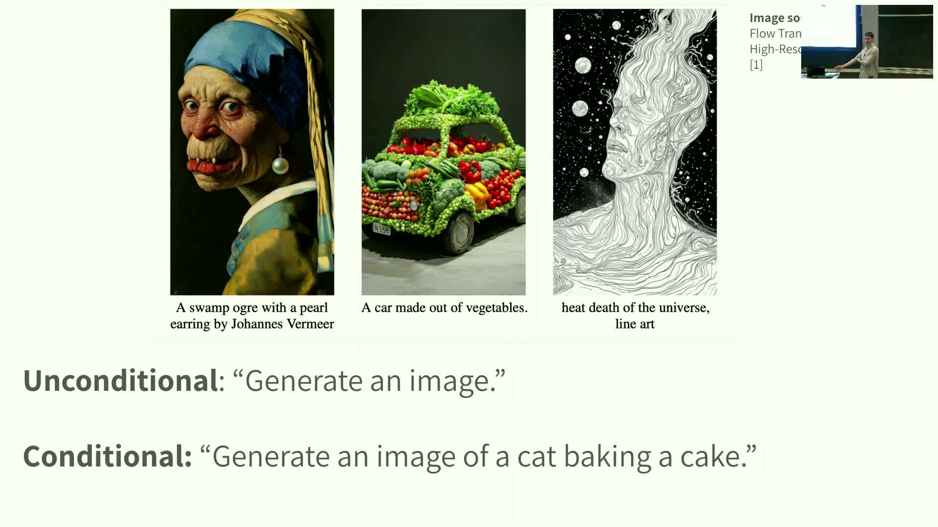
This segment formalizes terminology for guided generation and introduces the conditioning variable.
- Terminology:
- Replace unconditional with unguided.
- Replace conditional with guided.
- Replace unconditional with unguided.
- Conditioning variable:
- Denote the conditioning information by y (examples: text prompt, class label, MNIST digit label).
- Formally, guiding means conditioning on y, so marginals, vector fields, and scores become guided quantities conditioned on y.
- Denote the conditioning information by y (examples: text prompt, class label, MNIST digit label).
-
Notational change: prepend “guided” to previously unconditional objects and write the guided target as **p_data(x y)** with corresponding guided vector fields and scores.
- Clarification: y may be discrete or continuous depending on the task, and this setup prepares the training and sampling objectives in the guided context.
Guided conditional flow matching objective: fixed y and amortization over y
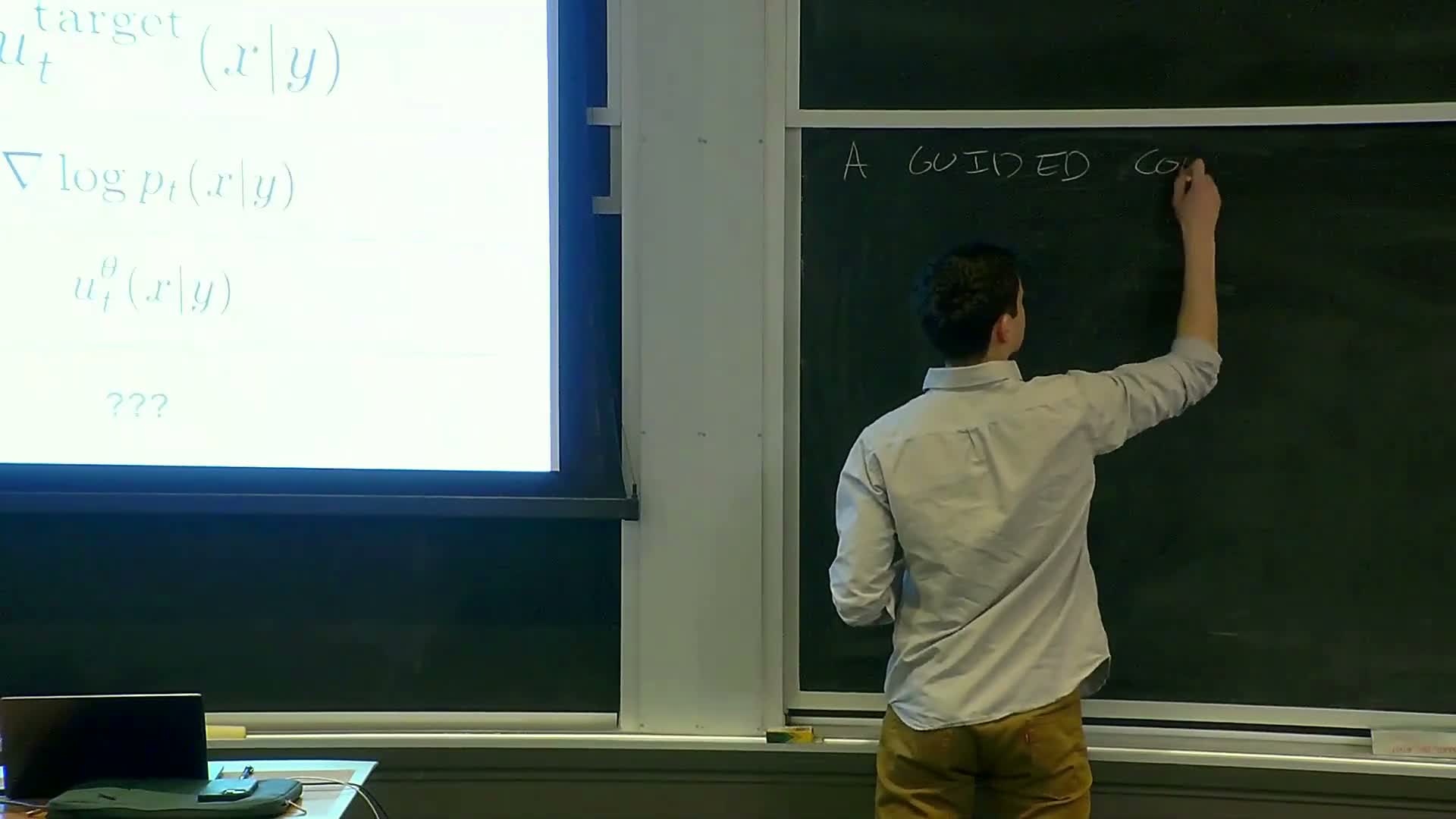
This segment constructs the guided conditional flow matching (LCFM) objective and explains amortization across y.
- Fixed-y training:
- Fix a specific y.
-
Regress the guided vector field **u_t^θ(x y)** onto the conditional target vector field using expectations over the guided probability path.
-
Sampling inside the expectation: sample t ∼ Uniform[0,1], sample **z ∼ p_init(z y)**, then sample **x ∼ p_t(x z,y)**, and minimize the squared error between model and target.
- Fix a specific y.
- Amortized conditional training:
- Let y vary and define a single loss that takes expectation over the joint data distribution (z,y).
- Practically this is implemented by a data loader that returns paired (image, prompt) examples.
- Let y vary and define a single loss that takes expectation over the joint data distribution (z,y).
- Result: conditional flow matching reduces to standard conditional training applied across the support of y, enabling a single amortized model to learn all conditionings.
Training and sampling with guided vector fields
This segment describes the practical training and sampling pipeline using the guided objective.
- Training:
-
Minimize the guided conditional flow matching loss across (z,y) pairs to learn **u_t^θ(x y)**.
-
- Sampling:
- Choose a prompt y.
- Initialize x ∼ p_init.
- Simulate the ODE from t = 0 to t = 1 using the trained conditional vector field.
- Choose a prompt y.
- SDE parallel: when training scores instead of vector fields, use the equivalent SDE formulation (see notes for details).
-
Theoretical guarantee: guided training + accurate numerical simulation recovers samples from **p_data(x y)** in the idealized limit.
- Practical deviation: practitioners often modify sampling (e.g., classifier-free guidance) to improve perceptual quality, at the cost of deviating from the exact guided sampler.
Introduction to classifier-free guidance and motivation
This segment introduces classifier-free guidance (CFG) as a practical sampling modification.
- Motivation: trade sample diversity for perceptual quality and stronger prompt adherence.
- Empirical discovery: scaling the contribution of the conditioning signal often yields samples that appear more faithful to prompts, even though the resulting vector field is no longer the exact guided field.
- Historical note: CFG is widely used in production models (including Stable Diffusion 3).
- Analytical setup: the forthcoming derivation is developed for Gaussian probability paths to build intuition, though the idea generalizes beyond Gaussians.
- Purpose: relate marginal vector fields and score functions on Gaussian paths to motivate CFG.
Gaussian conditional probability paths and relation between vector fields and scores
This segment defines Gaussian conditional probability paths and links vector fields to scores.
- Gaussian path definition:
-
p_t(x z) = Normal(alpha_t x, beta_t^2 I), with smooth monotonic functions alpha_t and beta_t satisfying endpoint constraints.
-
- Key algebraic relation:
-
The guided marginal vector field *u_t^(x y)** can be written in affine form: -
*u_t^(x y) = a_t x + b_t ∇_x log p_t(x y)**.
-
- The coefficients a_t and b_t have explicit expressions determined by derivatives of alpha_t and beta_t.
-
-
Implication: this relation lets us express guided vector fields using the score ∇_x log p_t(x y) and constants set by the Gaussian noise schedule — a foundation for the CFG derivation.
Bayes decomposition of the guided score and identification of a classifier term
This segment decomposes the guided marginal score using Bayes’ rule and identifies the classifier-like term.
- Bayes decomposition:
-
**∇_x log p_t(x y) = ∇_x log p_t(x) + ∇_x log p_t(y x)**.
-
- Substitution into the vector-field relation yields:
-
The guided vector field = unguided vector field + a term proportional to **∇_x log p_t(y x)**.
-
- Interpretation:
-
**∇_x log p_t(y x)** behaves like a classifier because it evaluates how likely a given x is under each y (e.g., class label).
- This term therefore carries the conditioning signal and is a natural target for amplification to strengthen adherence to the prompt during sampling.
-
Guidance scaling factor and constructing an amplified guided vector field
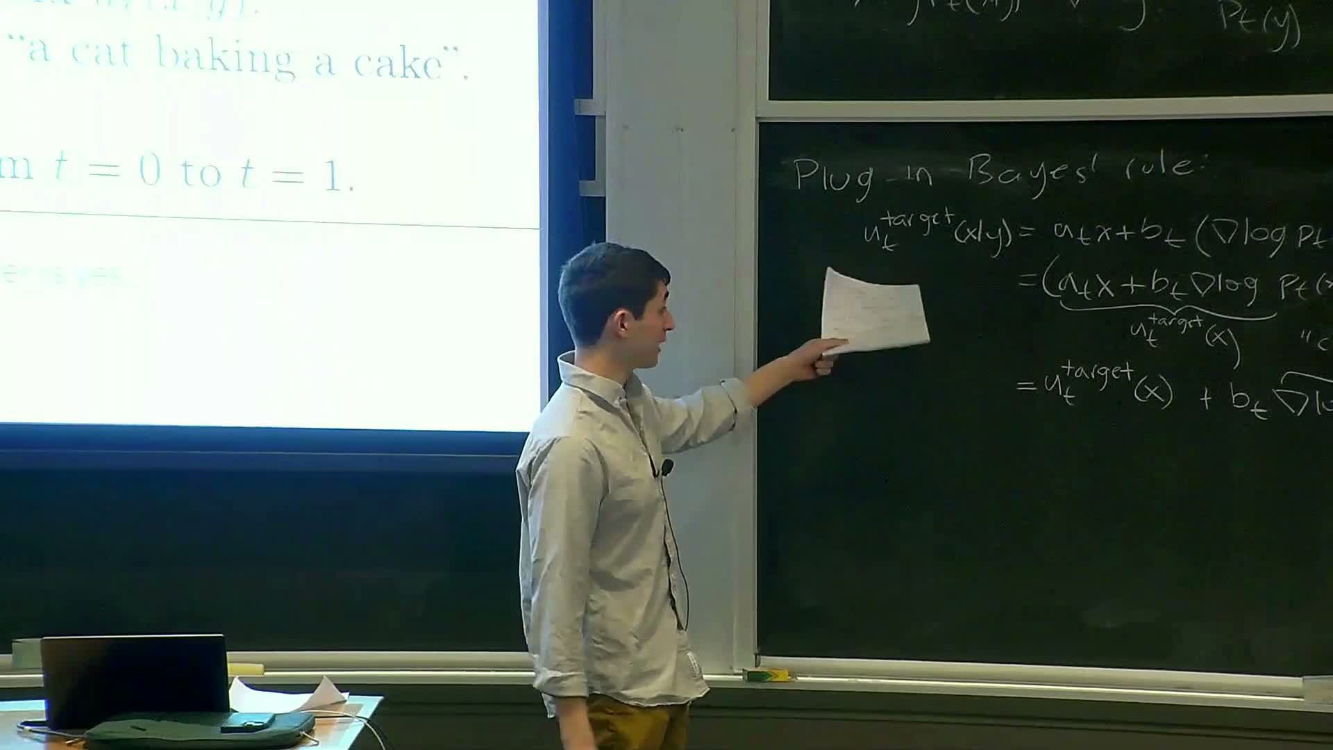
This segment introduces an explicit guidance scale to amplify the classifier-like term and gives intuition about its effect.
- Define a guidance scale w > 1 that multiplies the classifier-like term in the guided vector field.
- Modified vector field:
-
**ũ_t = u_t (unguided) + b_t w ∇_x log p_t(y x)**.
-
- Interpretation:
-
Scaling the classifier term concentrates sampling mass in regions that score highly under **p_t(y x), trading **diversity for perceptual fidelity (similar to low-temperature sampling).
-
- Notes:
- More principled classifier-based guidance methods exist, but CFG provides a simple and effective practical mechanism controlled by a single multiplicative hyperparameter w.
- More principled classifier-based guidance methods exist, but CFG provides a simple and effective practical mechanism controlled by a single multiplicative hyperparameter w.
Algebraic rearrangement to classifier-free guidance and single-model training with null token
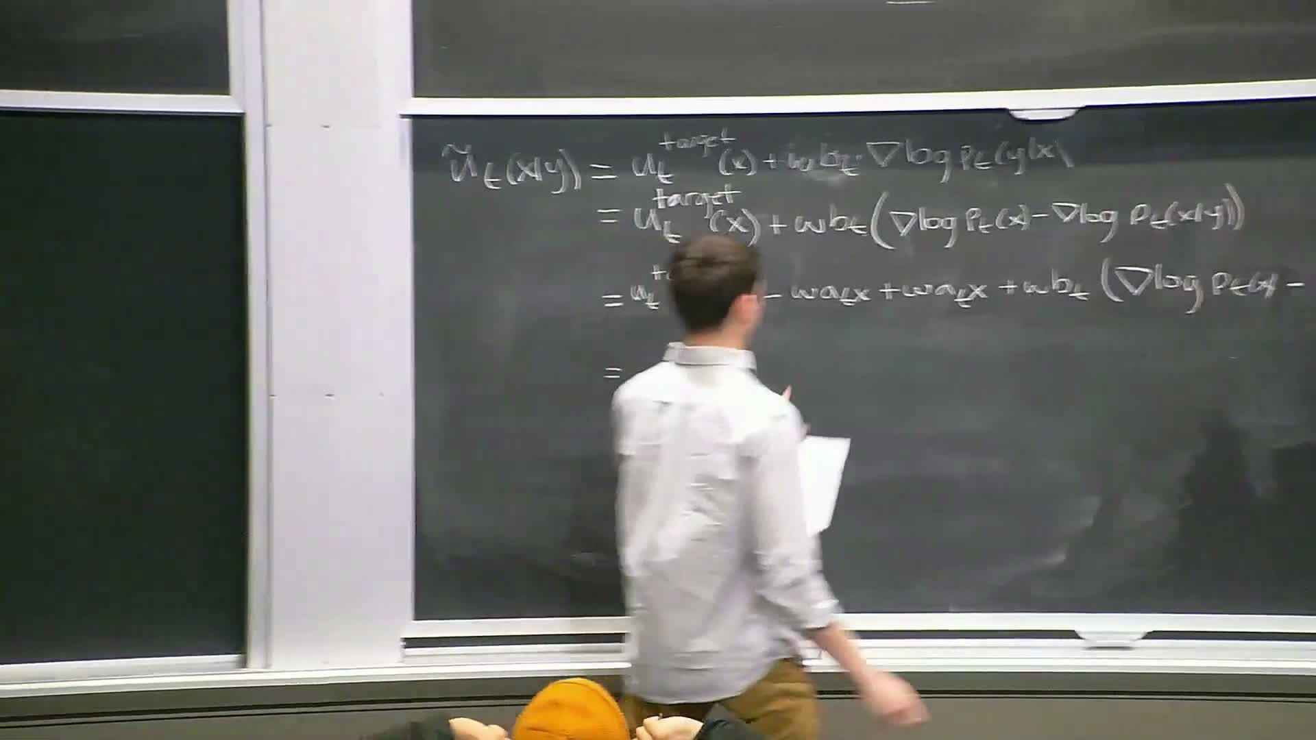
This segment algebraically rewrites the CFG-modified vector field and motivates the classifier-free training trick.
- Algebraic rearrangement yields the commonly used implementation form:
-
**ũ_t = (1 + w) u_t(x y) − w u_t(x null)**.
-
- Classifier-free training recipe:
-
Train a single model **u_t^θ(x y)** that can accept either a real conditioning y or a special null token.
- During training, randomly drop conditioning with probability p_drop so the model learns both guided and unguided behaviors.
-
- Inference:
- Use the same model twice (conditioned on y and on null) and combine outputs with scale w to implement CFG without an external classifier.
- Use the same model twice (conditioned on y and on null) and combine outputs with scale w to implement CFG without an external classifier.
- Benefit: efficient training and sampling with a single amortized conditional model that matches the algebraic CFG form used in practice.
Practical sampling with CFG and empirical MNIST example
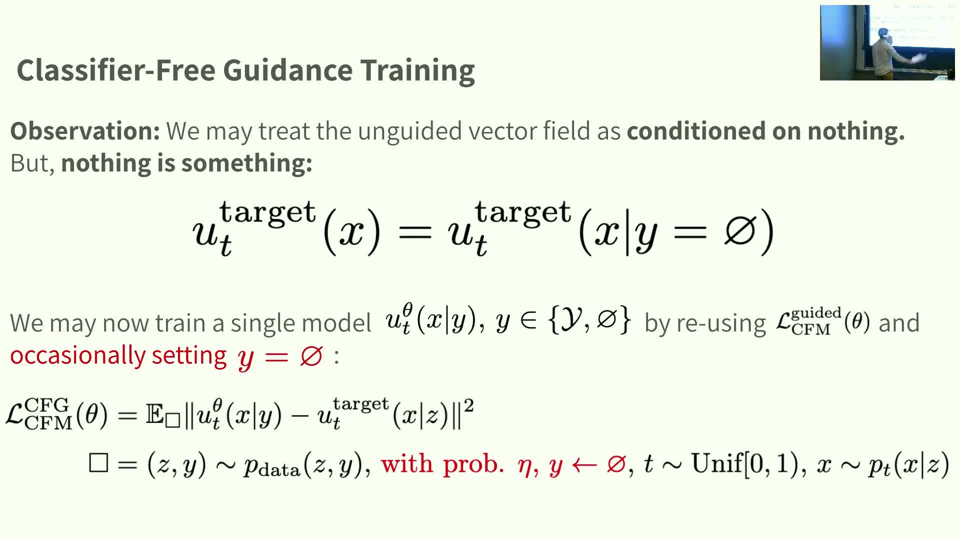
This segment describes the CFG sampling procedure and empirical behavior (MNIST demonstration).
- CFG sampling steps:
- Train the conditional model with occasional null conditioning.
- Select a prompt y (or null for unguided) and choose guidance scale w.
- Initialize x ∼ p_init and integrate the CFG-modified vector field ũ_t from t = 0 to t = 1 to produce samples.
- Train the conditional model with occasional null conditioning.
- Empirical observation (MNIST):
- Increasing w tends to improve perceptual quality (clearer digits) while reducing diversity across samples.
- Increasing w tends to improve perceptual quality (clearer digits) while reducing diversity across samples.
- Practical note:
- Although w > 1 deviates from the theoretically exact guided sampler, practitioners prefer CFG for subjectively sharper and more prompt-faithful results, and the null-token trick makes it simple to implement.
- Although w > 1 deviates from the theoretically exact guided sampler, practitioners prefer CFG for subjectively sharper and more prompt-faithful results, and the null-token trick makes it simple to implement.
Real-world CFG examples and discussion of classifier identity and effects
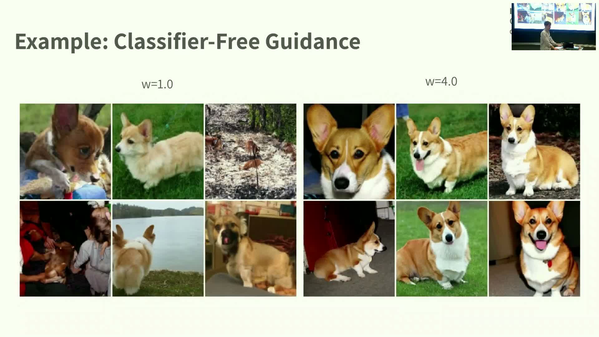
This segment shows real-world CFG examples and discusses intuition and open questions.
- Empirical examples:
- For image prompts (e.g., corgi photos), unguided or exact-guided sampling (w = 1) can produce plausible but weakly prompt-aligned images; increasing w yields more prompt-faithful and visually pleasing samples.
- For image prompts (e.g., corgi photos), unguided or exact-guided sampling (w = 1) can produce plausible but weakly prompt-aligned images; increasing w yields more prompt-faithful and visually pleasing samples.
- Clarification of the classifier term:
-
When y is a discrete class label, the classifier term is **p(y x)**; in CFG practice the conditional generative model itself typically supplies this term rather than an external classifier.
-
- Intuition for why boosting helps:
- Amplifying the classifier term acts like truncation or low-temperature sampling by concentrating probability mass into modes favored by the prompt.
- Amplifying the classifier term acts like truncation or low-temperature sampling by concentrating probability mass into modes favored by the prompt.
- Open questions:
- The precise theoretical justification for CFG and principled tuning of w remain active research areas.
- The precise theoretical justification for CFG and principled tuning of w remain active research areas.
Image data structure and why MLPs are insufficient for high-resolution images
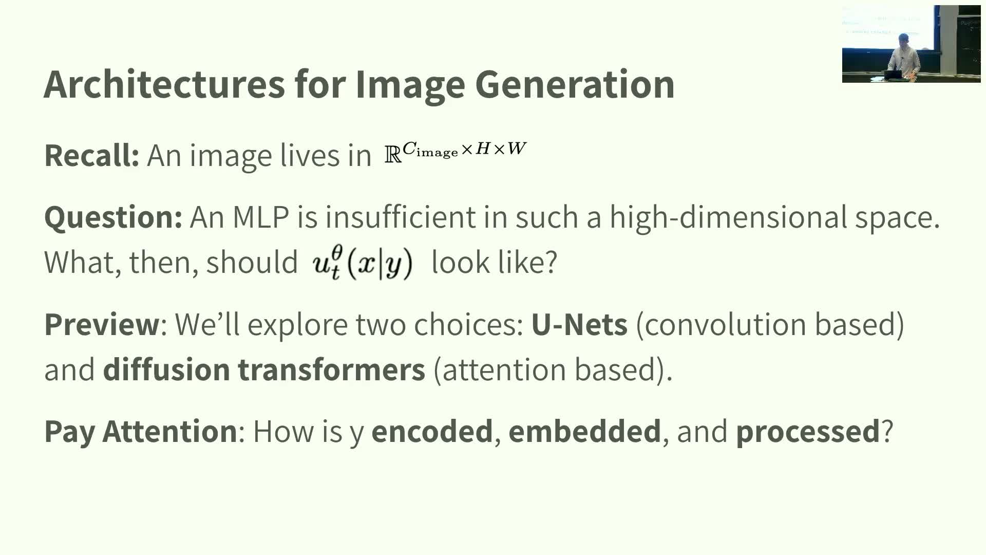
This segment defines images as tensors and motivates architecture choices for scaling to high-resolution images.
- Image representation:
- Images are tensors in R^{C × H × W}, with common channel conventions like RGB.
- Images are tensors in R^{C × H × W}, with common channel conventions like RGB.
- Why naive MLPs fail:
- Fully connected MLP parameterizations do not scale to large H, W and ignore important spatial inductive biases, making them inefficient for images.
- Fully connected MLP parameterizations do not scale to large H, W and ignore important spatial inductive biases, making them inefficient for images.
- Architectural desiderata for image generative models:
-
Parameter efficiency.
-
Spatial inductive bias to exploit locality and multi-scale structure.
-
Flexible conditioning mechanisms that align prompt embeddings with image features.
-
Parameter efficiency.
- Practical choices:
-
Convolutional UNets and attention-based diffusion Transformers are two common, effective architectures that meet these criteria.
-
Convolutional UNets and attention-based diffusion Transformers are two common, effective architectures that meet these criteria.
UNet architecture overview for diffusion/flow models
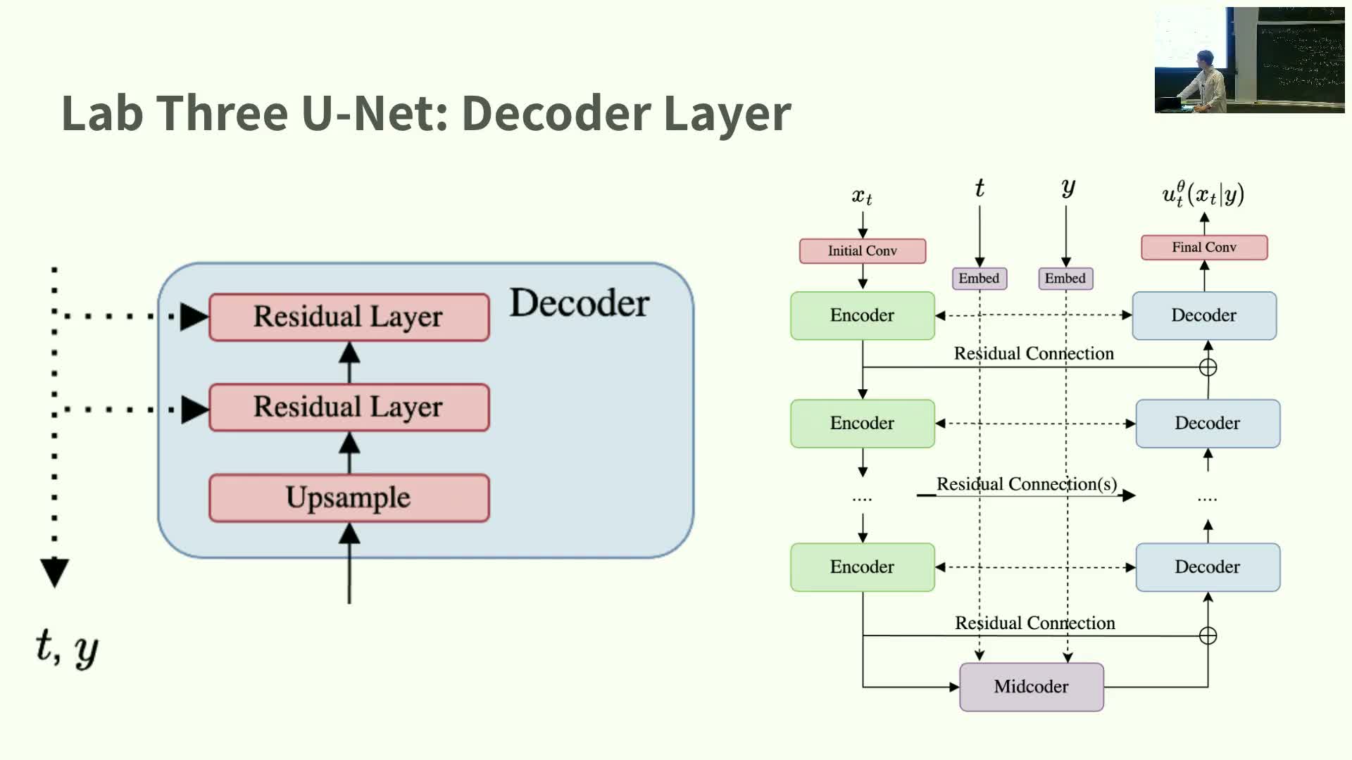
This segment gives a high-level description of the UNet architecture used in diffusion and flow models.
- UNet topology:
-
Downsampling encoder path: increases channels while reducing spatial resolution.
-
Mid-level bottleneck: preserves spatial size while processing coarse features.
-
Upsampling decoder path: restores spatial resolution.
-
Skip connections: pass encoder features directly to corresponding decoder layers for multi-scale fusion.
-
Downsampling encoder path: increases channels while reducing spatial resolution.
- Conditioning and time injection:
-
Time embeddings (sinusoidal or Fourier) and conditioning embeddings for y are injected into residual blocks, typically by projecting embeddings to the channel dimension and adding them channel-wise between convolutions.
-
Time embeddings (sinusoidal or Fourier) and conditioning embeddings for y are injected into residual blocks, typically by projecting embeddings to the channel dimension and adding them channel-wise between convolutions.
- Building blocks:
- Residual layers composed of convolution → normalization → activation are stacked, with variants differing in normalization type, channel counts, and block counts.
- Residual layers composed of convolution → normalization → activation are stacked, with variants differing in normalization type, channel counts, and block counts.
- Core benefit: the U-shaped topology enables efficient multi-scale feature processing essential for high-quality image generation.
Residual layer internals and conditioning injection in UNet
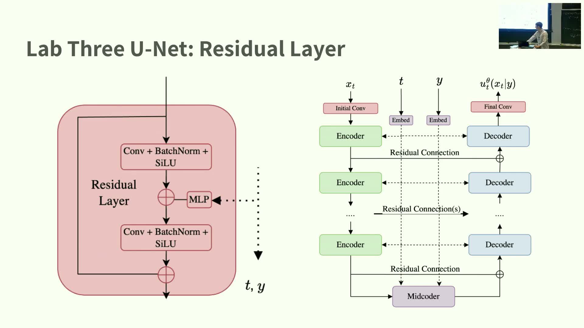
This segment describes the internal structure of a UNet residual block and how conditioning is injected.
- Residual block structure:
- A residual shortcut plus two convolutional layers, each with normalization and nonlinear activation.
- A residual shortcut plus two convolutional layers, each with normalization and nonlinear activation.
- Conditioning injection:
- Map time and conditioning embeddings through an MLP to match the block’s channel dimensionality.
- Add these projected embeddings channel-wise to intermediate activations between convolutional layers.
- Map time and conditioning embeddings through an MLP to match the block’s channel dimensionality.
- Practical points:
- Channel-wise addition is computationally efficient and lets the block modulate processing based on timestep and prompt.
- Stacked residual blocks plus downsampling/upsampling implement the full UNet.
- Channel-wise addition is computationally efficient and lets the block modulate processing based on timestep and prompt.
Diffusion Transformer (patch-based attention)
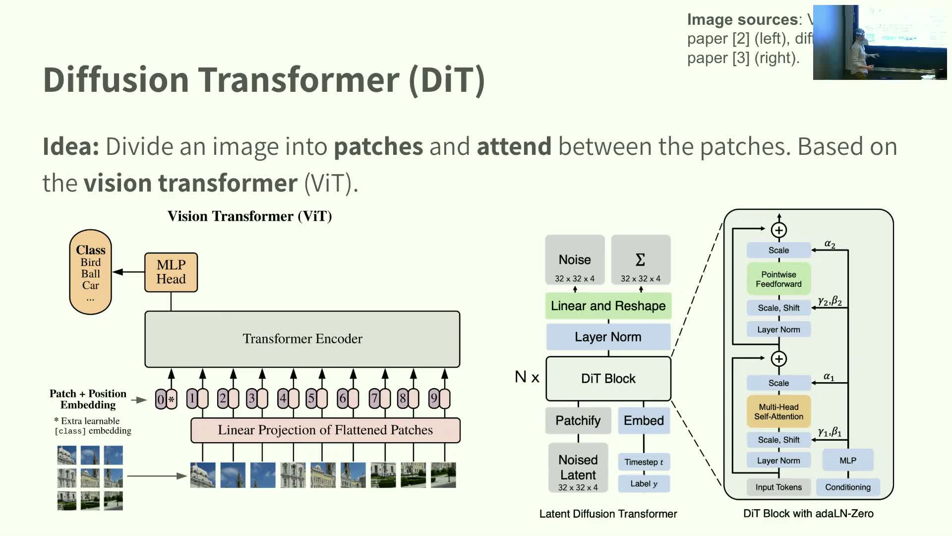
This segment presents the diffusion Transformer alternative for image generation.
- Key idea: treat the image as a sequence of patch tokens, borrowing the Vision Transformer (ViT) paradigm.
- Architecture:
- Partition the image into patches, embed each patch to a feature vector, and process the token sequence with Transformer attention blocks.
-
Positional encodings provide spatial awareness; multi-head self-attention models long-range dependencies and replaces local convolutional receptive fields.
- Partition the image into patches, embed each patch to a feature vector, and process the token sequence with Transformer attention blocks.
- Adaptation to diffusion tasks:
- Diffusion Transformers predict noise or denoised outputs per patch token and integrate time and conditioning embeddings into attention blocks.
- Diffusion Transformers predict noise or denoised outputs per patch token and integrate time and conditioning embeddings into attention blocks.
- Benefit: attention-based parameterizations scale to model global structure and long-range interactions useful for high-fidelity image synthesis.
Latent-space modeling and the latent diffusion design pattern
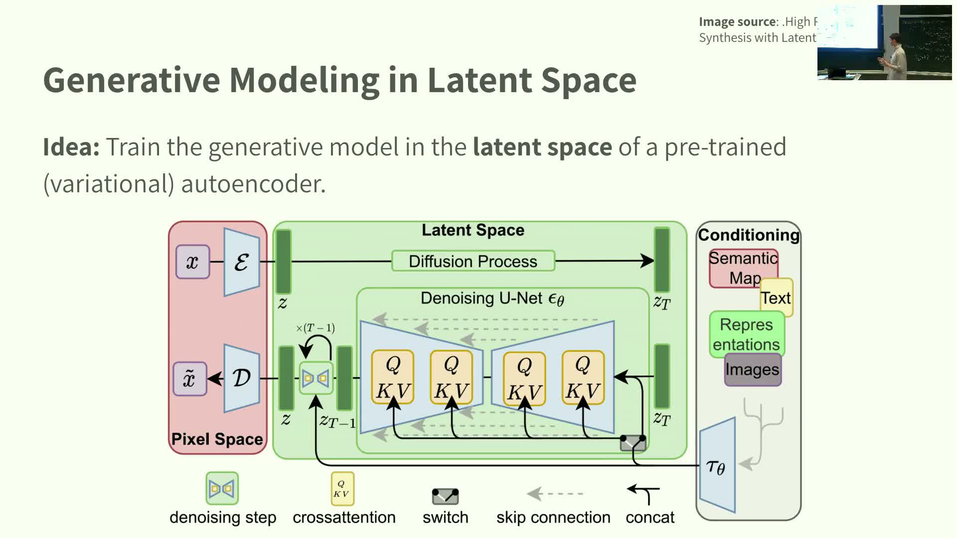
This segment explains the latent-space design pattern used in many modern pipelines.
- Latent-space recipe:
- Pretrain an encoder/decoder (e.g., autoencoder or VAE) that compresses images into a lower-dimensional latent space.
- Train the generative diffusion or flow model in that latent space instead of raw pixels.
- At sampling time, generate latents and decode them to full-resolution images.
- Pretrain an encoder/decoder (e.g., autoencoder or VAE) that compresses images into a lower-dimensional latent space.
- Rationale:
- Latents remove imperceptible high-frequency detail, reduce dimensionality (cheaper computation), and focus the generator on perceptually relevant structure.
- Latents remove imperceptible high-frequency detail, reduce dimensionality (cheaper computation), and focus the generator on perceptually relevant structure.
- Practical note: latent diffusion is widely used; modern pipelines commonly combine pretrained encoders with UNet or Transformer generative backbones operating in latent coordinates.
Stable Diffusion 3 case study and multimodal conditioning

This segment surveys Stable Diffusion 3 as an instantiation of the described design patterns.
- Key components:
-
Latent diffusion backbone operating in compressed image latents.
- Large conditional UNet or multimodal diffusion Transformer as the expressive generative backbone.
- Pretrained encoders (e.g., CLIP, T5) to produce robust text embeddings for cross-modal alignment.
-
Classifier-free guidance to steer generation during sampling.
-
Latent diffusion backbone operating in compressed image latents.
- Practical integration:
- Stable Diffusion 3 parameterizes u_t with a highly expressive conditional model trained with conditional flow matching objectives.
- It integrates image-text embeddings (CLIP) and sequence-level language model embeddings inside attention, enabling richer prompt context and high-resolution, prompt-aligned synthesis.
- Stable Diffusion 3 parameterizes u_t with a highly expressive conditional model trained with conditional flow matching objectives.
Course logistics and transition to guest lecture
This segment covers course logistics and transitions to a guest speaker.
- Logistics reminders:
- Upcoming lectures and guest talks (robotics, protein design).
- Lab submission deadlines and office hours schedule/location.
- Upcoming lectures and guest talks (robotics, protein design).
- Transition: introduce the guest presenter (affiliation and research focus) who will discuss reward fine-tuning for flow and diffusion models.
- Purpose: close the instructor portion and set expectations for the guest lecture that follows.
Guest lecture introduction: reward fine-tuning for flow and diffusion models
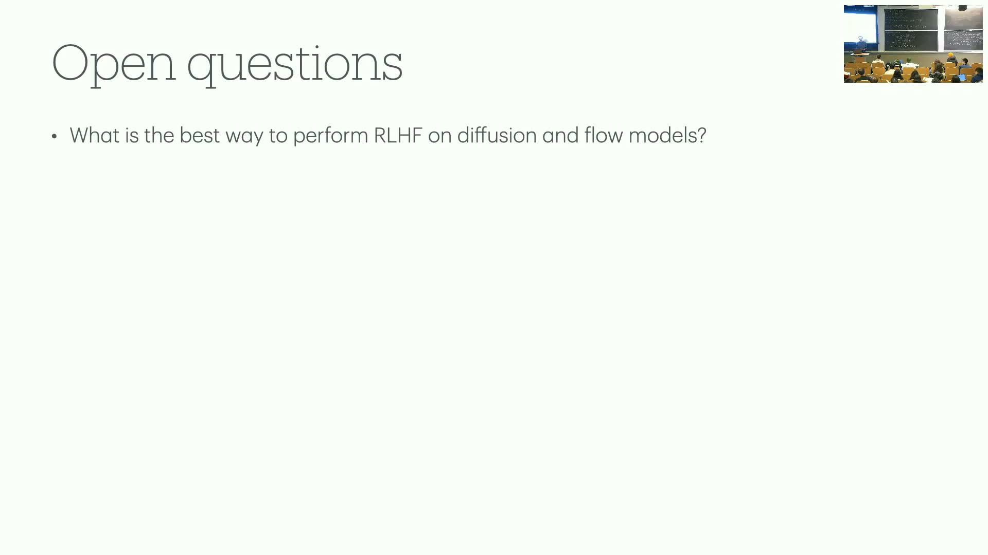
This segment frames the guest lecture on reward fine-tuning (RF) for generative diffusion and flow models.
- Problem statement:
- Given a pretrained base model p_base (often conditional, e.g., text-to-image) and a reward model trained from human preferences or other signals, how should we modify the generative model to optimize a reward objective?
- Given a pretrained base model p_base (often conditional, e.g., text-to-image) and a reward model trained from human preferences or other signals, how should we modify the generative model to optimize a reward objective?
- RF objective:
- Modify the pretrained generator so it samples from p_star ∝ p_base(x) exp(R(x)), i.e., bias generation toward higher reward while staying close to the base distribution.
- Modify the pretrained generator so it samples from p_star ∝ p_base(x) exp(R(x)), i.e., bias generation toward higher reward while staying close to the base distribution.
- Connections:
- RF relates to stochastic optimal control and contrasts with RL-style approaches used for language models (e.g., PPO, DPO).
- Continuous-time structure of diffusion/flow models opens alternative algorithmic opportunities for RF.
- RF relates to stochastic optimal control and contrasts with RL-style approaches used for language models (e.g., PPO, DPO).
Fine-tuning objective as KL-regularized optimization and SDE/flow connections
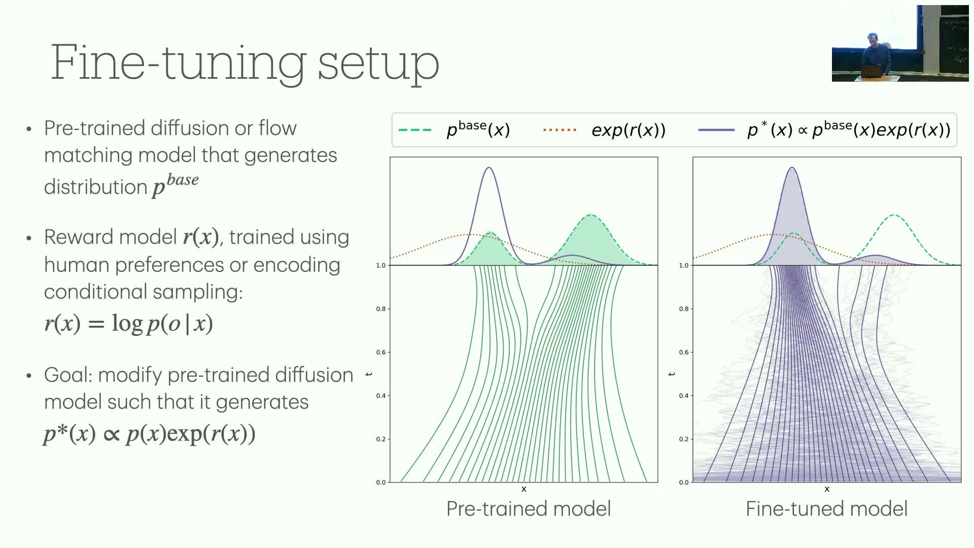
This segment connects RF to a KL-regularized optimization and the path-space control perspective.
- Optimization viewpoint:
- Target distribution p_star maximizes expected reward with a penalty for deviating from p_base, i.e., a KL-regularized objective.
- Target distribution p_star maximizes expected reward with a penalty for deviating from p_base, i.e., a KL-regularized objective.
- Path-space control formulation:
- Cast the problem as minimizing expected negative reward plus a control cost proportional to the KL divergence between controlled and base path measures.
- The optimal controlled path measure is proportional to the base path measure multiplied by exp(reward) (up to normalization).
- Cast the problem as minimizing expected negative reward plus a control cost proportional to the KL divergence between controlled and base path measures.
- Practical implication:
- Implementing this in diffusion/flow frameworks requires choosing compatible noise schedules and dynamics so the control problem is tractable.
- Implementing this in diffusion/flow frameworks requires choosing compatible noise schedules and dynamics so the control problem is tractable.
Flow matching, SDE sampling equivalence, and the role of arbitrary noise schedules
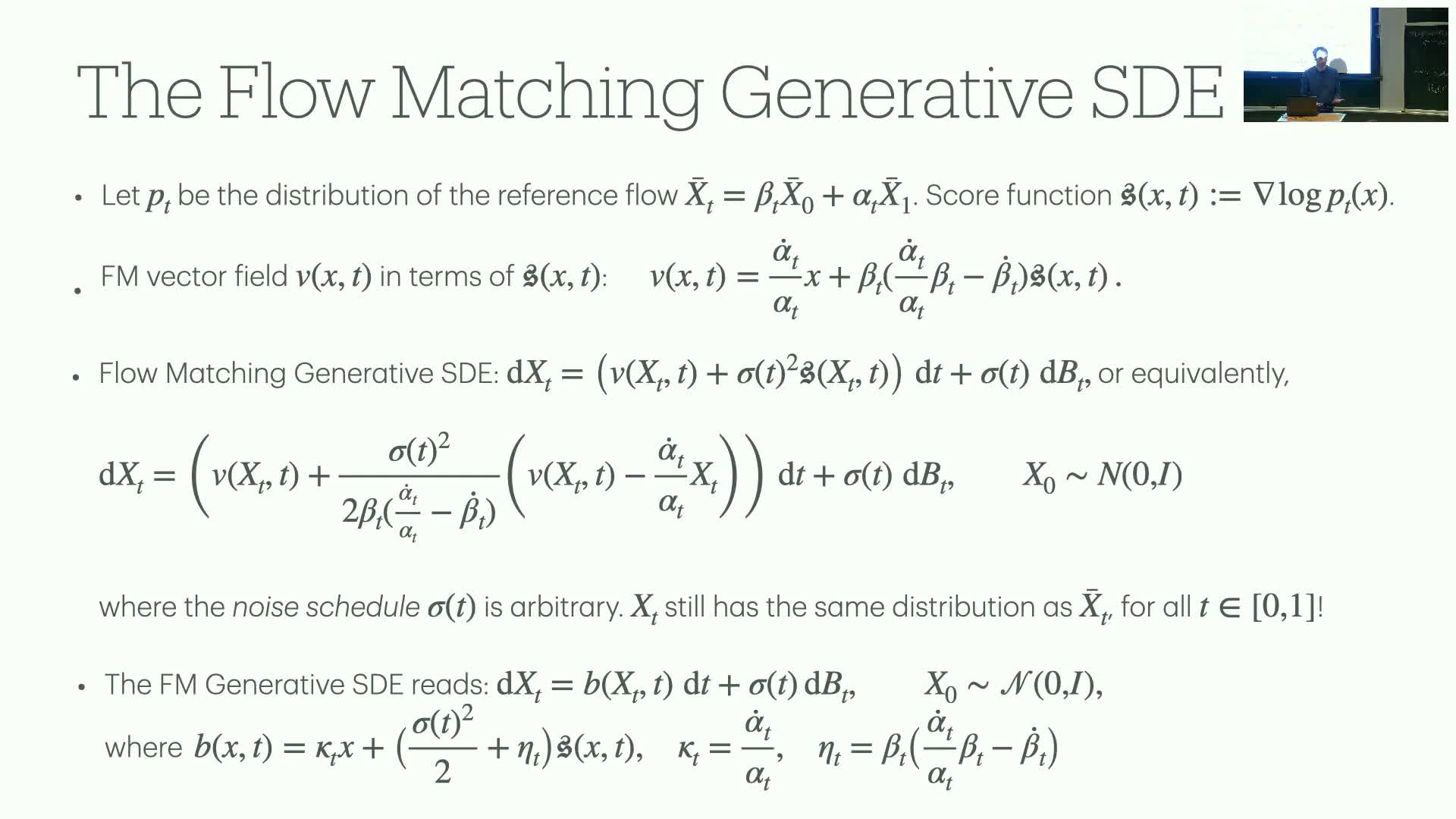
This segment reviews flow matching and its SDE counterpart and connects them to fine-tuning considerations.
- Flow matching:
- A learned flow vector field yields a generative ODE whose marginals match the reference marginals when trained exactly.
- A learned flow vector field yields a generative ODE whose marginals match the reference marginals when trained exactly.
- SDE alternative:
- One can sample the same marginals via an SDE by combining an arbitrary diffusion coefficient with a score-based corrective drift.
- One can sample the same marginals via an SDE by combining an arbitrary diffusion coefficient with a score-based corrective drift.
- Practical implication for RF:
- Flow models can be sampled either by ODE solvers or SDE samplers; choosing an arbitrary noise schedule in the SDE can be leveraged during fine-tuning.
- However, the fine-tuning noise schedule must be chosen carefully to maintain equivalence to the desired target distribution — this underpins results about memoryless noise schedules required for principled fine-tuning.
- Flow models can be sampled either by ODE solvers or SDE samplers; choosing an arbitrary noise schedule in the SDE can be leveraged during fine-tuning.
Stochastic optimal control interpretation of fine-tuning and necessity of memoryless noise schedules
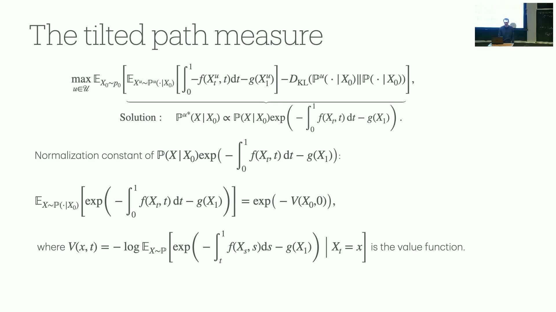
This segment develops the stochastic optimal control viewpoint for reward fine-tuning and states the memoryless schedule theorem.
- Control formulation:
- Treat the difference between the fine-tuned drift and the base drift as a control, and form an objective trading expected terminal reward against an integrated quadratic control cost along trajectories.
- Treat the difference between the fine-tuned drift and the base drift as a control, and form an objective trading expected terminal reward against an integrated quadratic control cost along trajectories.
- Theoretical result:
- The optimal controlled path measure equals the base path measure multiplied by the exponential of rewards — but to ensure the final-time marginal equals p_star (independent of the initial state), the generative process must satisfy a memoryless property.
- The optimal controlled path measure equals the base path measure multiplied by the exponential of rewards — but to ensure the final-time marginal equals p_star (independent of the initial state), the generative process must satisfy a memoryless property.
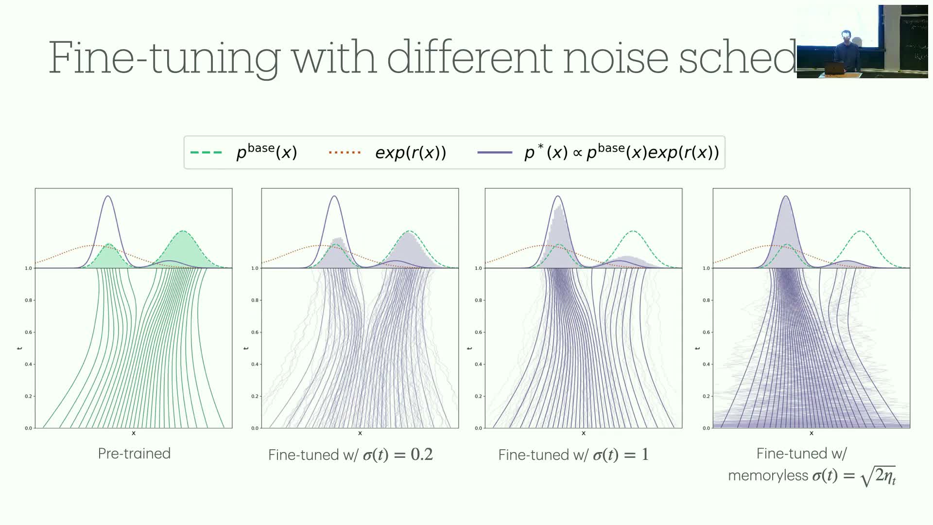
- Practical theorem:
- Choosing a specific memoryless noise schedule (for the Gaussian path parameterization, sigma_t^2 = 2 a_t) makes fine-tuning implementable and targets p_star correctly.
- Choosing a specific memoryless noise schedule (for the Gaussian path parameterization, sigma_t^2 = 2 a_t) makes fine-tuning implementable and targets p_star correctly.
- Empirical note:
- Deviating from the memoryless schedule produces biased or suboptimal fine-tuned distributions in practice.
- Deviating from the memoryless schedule produces biased or suboptimal fine-tuned distributions in practice.
Agent method for solving the control problem and adjoint/agent matching
This segment describes computational methods for solving the stochastic optimal control problem for fine-tuning, focusing on agent-based approaches.
- Two equivalent algorithmic views:
- Direct policy-gradient–like viewpoint: optimize a parametric control network by sampling rollouts and optimizing the expected control objective via backpropagation through time.
-
Adjoint / agent-matching regression viewpoint: regress the control against an adjoint (costate) that satisfies a backward ODE; at optimum the control equals minus the gradient of the value function scaled by sigma^T.
- Direct policy-gradient–like viewpoint: optimize a parametric control network by sampling rollouts and optimizing the expected control objective via backpropagation through time.
- Practical considerations:
- Adjoint formulations can be implemented via additional ODEs and often reduce variance if designed carefully.
- A modified agent-matching variant that cancels high-variance terms performed best in the authors’ experiments, indicating variance control is critical for practical RF.
- Adjoint formulations can be implemented via additional ODEs and often reduce variance if designed carefully.
- Takeaway: both rollout-based and adjoint-regression approaches are viable; careful variance reduction and schedule choices are key for successful reward fine-tuning in continuous-time generative models.
Enjoy Reading This Article?
Here are some more articles you might like to read next: