Less is More - Recursive Reasoning with Tiny Networks
About the paper
Less is More: Recursive Reasoning with Tiny Networks, by Alexia Jolicoeur-Martineau, introduces this Tiny Recursive Model (TRM). It learns from paired problems and solutions, without intermediate reasoning labels. The idea matters because it separates how many parameters a model stores from how much computation it performs: a small learned module can support a long process of refinement. Its intermediate work takes place in continuous hidden states, and training teaches those updates through their effect on the predicted answer. The paper shows an impressive result: a tiny model with only 5-million-parameters can achive 87.4% of Sudoku-Extreme dataset, a significant boost from 55.0% with 27-million-parameter model (HRM).
This post follows that computation from input embeddings to answer predictions, explains how deep supervision trains repeated refinement, and connects the equations to the implementation. Along the way, we will see what TRM changes from HRM, how it relates to looped Transformers such as LoopLM, and what would need to change to apply it to biomedical relation extraction.
TL;DR
- Architecture: reuse a small network to refine an answer. TRM maintains an embedded input \(x\), a candidate-answer state \(y\), and an auxiliary reasoning state \(z\). One shared two-layer network repeatedly updates \(z\), then revises \(y\); an output head reads \(y\) to predict all output positions in parallel. The network can use self-attention or token-mixing MLPs.
- Training: supervise refinement in manageable steps. Each supervision step runs several reasoning cycles, retaining gradients through the final complete cycle. The model receives an answer loss and carries detached states into the next step, allowing repeated refinement without backpropagating through the entire history.
- Halt prediction: learn when an example has received enough computation. The default halt head predicts whether every supervised output token is correct, using binary classification rather than a bootstrapped Q-learning continue target. Learned halting controls training; evaluation uses the full configured budget, normally 16 supervision steps.
- Batch slots: different example lifetimes, synchronized GPU work. Each training iteration runs one supervision step for every slot in a fixed-size batch, followed by a shared optimizer update. Previously halted slots accept new examples and reset their states; unfinished examples retain their inputs, labels, and states. Examples can therefore receive different numbers of updates while GPU execution stays batched. The benefit is earlier admission of new examples, rather than a shorter inner computation for each batch step.
Sources: TRM method, halting and batch-slot implementation, and batched training loop.
From HRM to TRM
TRM builds on the Hierarchical Reasoning Model (HRM), whose distinctive feature is two recurrent modules operating at different timescales. A low-level module updates its hidden state several times while the high-level state stays fixed. The high-level module then incorporates the low-level result and supplies context for the next cycle. The two modules have separate networks and weights; predictions are read from the high-level state. The authors interpret these roles as detailed processing and higher-level planning, although the hidden states are not explicit, readable plans. HRM, Section 2
HRM made this approach worth studying through its task-specific Sudoku, maze, and ARC results with roughly 27M parameters, trained without language-model pretraining or intermediate reasoning labels. It showed that substantial computation could happen inside a compact recurrent model. TRM investigates how much of HRM’s machinery is needed: it preserves repeated refinement and supervision across steps while simplifying the networks, gradient computation, and halting objective. HRM, Section 3.2; TRM, Sections 3–4
TRM keeps two states but gives them a simpler interpretation:
| Symbol | Meaning | Connection to the implementation |
|---|---|---|
| \(x\) | Embedded input question; available throughout refinement | Token, puzzle, and position information |
| \(y\) | Current answer representation; the output head reads this state | z_H |
| \(z\) | Auxiliary reasoning state; carries information used to revise the answer | z_L |
Here \(y\) is a continuous tensor, not the ground-truth answer and not a sequence of sampled tokens. Decoding it produces the current prediction. The two recurrent states start from initialization vectors and are then carried across refinement steps. In the official implementation, those initialization vectors are fixed random buffers broadcast across positions; they contain no solution information.
The important architectural change is that one shared network updates both states. TRM also backpropagates through a complete final reasoning cycle, simplifies the halt predictor, and uses an exponential moving average of the weights. These choices separate the method from the biological hierarchy and fixed-point interpretation used to motivate HRM. Paper, Section 4
One Reasoning Cycle: Think, Then Revise
Let \(f_\theta\) be the shared network and let \(n\) denote the number of reasoning-state updates. One cycle first holds the current answer \(y\) fixed while updating \(z\):
The cycle then revises the answer using the resulting reasoning state:
All three tensors have compatible shape \([B,L+P,D]\): batch size \(B\), token length \(L\), puzzle-prefix length \(P\), and hidden width \(D\). The additions are elementwise; the network’s attention or token-mixing layers exchange information between positions. The input \(x\) is explicitly injected during the reasoning updates. Its influence reaches the answer update through \(z\), even though \(x\) is not added again at that point.
Why retain both states? The answer state \(y\) provides a persistent candidate to improve, while the reasoning state \(z\) provides additional memory that does not have to be immediately decodable into an answer. This division is an architectural choice, not a guarantee that each hidden vector corresponds to a human-interpretable deduction.
Why can one network update both states? Both operations transform a hidden-width tensor into another tensor of the same shape, and their inputs already differ: refining \(z\) uses \(x+y+z\), while revising \(y\) uses \(y+z\). The author’s rationale is that this different conditioning may let one network learn both operations. The two states retain distinct roles even when their updates share parameters; information about \(x\) still reaches the answer update through the states.
The paper tests this choice in a Sudoku-Extreme ablation. The shared MLP model reaches 87.4% accuracy with 5M parameters, compared with 82.4% with 10M parameters for separate networks at the same effective depth. Sharing therefore reduces parameter count and improves generalization in that experiment, while keeping the number of network applications unchanged. The comparison supports this design choice for the tested setting; it does not isolate why sharing helps or establish that separate modules are always worse. Section 4.3 and Table 1
In the code below, net represents the shared reasoning module, including its position handling. This is the same computation as L_level(z_L, z_H + input_embeddings) followed by L_level(z_H, z_L) in the official implementation.
def reasoning_cycle(net, x, y, z, n):
    for _ in range(n):
        z = net(x + y + z)
    y = net(y + z)
    return y, z
How does a hidden answer become a prediction? The recursion above returns continuous vectors. An output head is a separate learned linear layer that reads each answer vector and produces one score for every possible output token. These unnormalized scores are called logits. In the official implementation, this layer is named lm_head; it maps hidden width \(D\) to vocabulary size \(V\) using a weight matrix \(W_{\mathrm{out}}\in\mathbb R^{V\times D}\) and no bias.
For example \(b\) and output position \(i\in\{0,\ldots,L-1\}\), the readout after a reasoning cycle is
Here \(P\) skips the puzzle-prefix positions, \(a_{bi,v}\) is the score for token \(v\), and \(\hat t_{bi}\) is the token with the highest score. The same output-head weights are used at every position. In Sudoku, this produces scores for all cells at once; selecting the largest score at each cell yields the proposed grid. The code below reads the current \(y\) after the refinement cycles, with output_head standing for the implementation’s lm_head:
# y: [B, L + P, D]; prefix_len is P.
logits = output_head(y)[:, prefix_len:]  # [B, L, V]
predicted_tokens = logits.argmax(dim=-1)  # [B, L]
The prediction loss is computed from the logits, allowing gradients to reach the output head and the reasoning network. The discrete argmax is used to inspect predictions and measure correctness; it is not the path through which the answer loss backpropagates. Further refinement carries the continuous \(y,z\) states forward. This is supervised structured prediction with all output positions decoded in parallel. The later relation-extraction example adapts the readout by supervising a relation-label position. Output-head definition and readout
Deep Recursion and Deep Supervision
There are three different loop counts to keep separate:
| Loop | What happens? | Configuration name |
|---|---|---|
| \(n\) reasoning updates | Revise \(z\) repeatedly before one revision of \(y\) | L_cycles |
| \(T\) complete cycles | Repeat the entire think–revise operation within one supervision step | H_cycles |
| Up to \(N_{sup}\) supervision steps | Carry the states forward and apply another prediction loss | halt_max_steps |
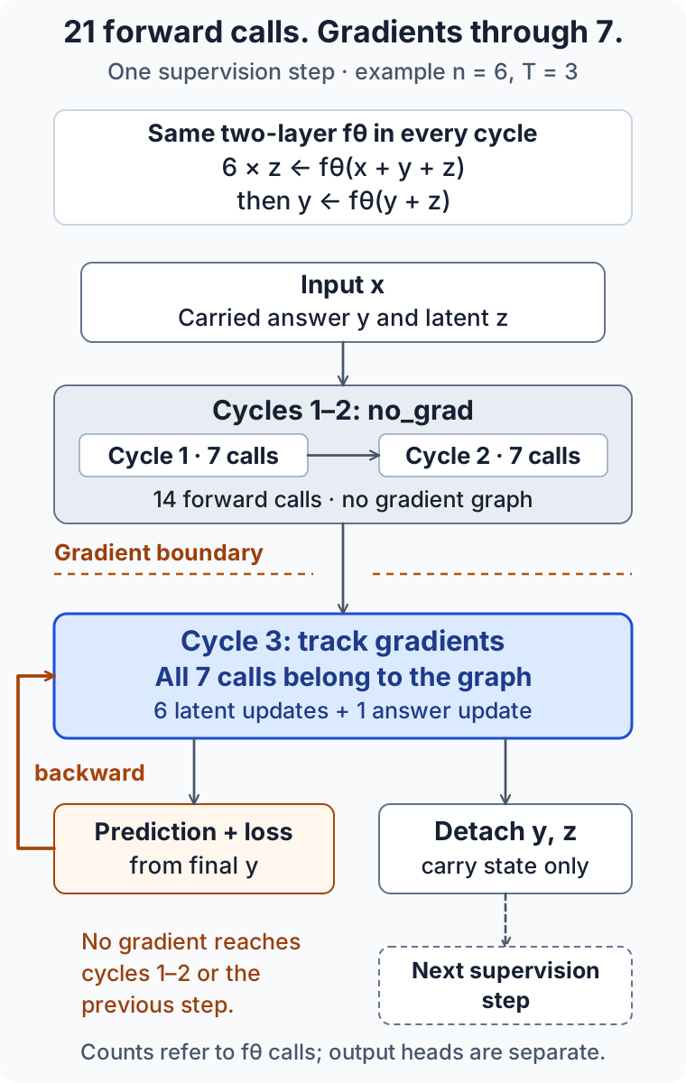
During training, the first \(T-1\) cycles run under torch.no_grad(). They produce a more developed starting state without retaining their activation graphs. The final cycle runs with gradients through all \(n+1\) network calls. A loss then supervises the decoded answer. Before the next supervision step, both recurrent states are detached, preserving their values while cutting the gradient connection to earlier steps.
This is a deliberately truncated gradient computation. It does not differentiate through the complete history, and it does not require the states to reach a mathematical fixed point. The model learns to improve the states encountered at the start of the gradient-tracked cycle. Improvement is the training objective; individual refinements are not guaranteed to increase accuracy.
The diagram shows these boundaries for the Sudoku setting \(n=6,T=3\). The same weights are used throughout; only the last cycle retains an activation graph for backpropagation.
For a network with \(d\) layers, the number of layer applications in one supervision step is
With \(d=2,n=6,T=3\), this gives 42 forward layer applications, of which 14 belong to the gradient-tracked final cycle. Running all 16 supervision steps gives up to 672 layer applications. These are repeated uses of the same two layers, not 672 independently parameterized layers. Increasing \(T\) adds forward computation; increasing \(n\) also lengthens the graph that must be retained during the last cycle. This explains why a tiny model can still have substantial runtime and activation-memory costs.
For the layer count, use the released TRM configuration: it sets L_layers=2. The existing architecture illustration in Main process is labeled 4x, which does not match this two-layer configuration.
Learning the Answer and When to Halt
Halting controls how many supervision steps a training example receives. The equations above describe the work inside one supervision step: \(d\), \(T\), and \(n\) are fixed, so each active example incurs \(dT(n+1)\) forward reasoning-layer applications, with \(d(n+1)\) tracked for gradients. If example \(b\) remains active for \(S_b\) supervision steps, its total counts are \(S_b dT(n+1)\) and \(S_b d(n+1)\), respectively. It participates in \(S_b\) separate batch-level backward passes and optimizer updates; the model does not backpropagate through that example’s entire history as one graph. For \(d=2,T=3,n=6\), stopping after two steps gives 84 forward layer applications, while running all 16 gives 672. The halt predictor decides when to stop revisiting an example and release its batch slot for new data, subject to exploration and the step limit. This matters because always using the maximum budget can spend many updates on already-correct answers, reducing the number of distinct examples seen within a fixed training budget. Halting changes how long an example occupies its slot, while each supervision step retains the same inner-loop computation. Training halting and batch-slot replacement
Let \(\tilde{y}_{bi}\) be the correct token at position \(i\) of example \(b\), and let \(m_{bi}\) indicate whether that position is supervised. A token-prediction loss averages the negative log-probability across each example’s valid positions:
The halt head predicts whether every supervised token is already correct. If \(c_b\) is that binary correctness target and \(q_b\) is the halt logit, the default implementation uses
The correctness target is computed from detached argmax predictions. It provides supervision for the halt head; gradients do not propagate through the discrete correctness test. During training, a positive halt logit can release an example’s batch slot for a new problem, subject to exploration and the maximum step count. During evaluation, the reference code always runs the configured maximum number of steps, normally 16. Paper, Section 4.6; model and ACT wrapper
A terminology note for the Q-Learning walkthrough below: the code retains HRM names such as q_head and q_continue_logits. However, TRM’s default no_ACT_continue=True removes the bootstrapped continue target and its extra model pass. The default halt objective above is supervised binary classification. The halt-versus-continue discussion describes the HRM-style alternative retained in the implementation, rather than a requirement for TRM.
The following educational PyTorch pseudocode shows one supervision step. embed_inputs, net, output_head, and q_head are adapters for the corresponding model components; prefix_len removes puzzle-prefix positions from token predictions. The example uses ordinary softmax cross-entropy to expose the training flow. The released configuration instead selects Stablemax cross-entropy, which normalizes a positive piecewise transformation of logits rather than their exponentials; reproducing the experiments requires that configured loss. Loss implementation
import torch
import torch.nn.functional as F


def supervision_step(model, batch, state, n=6, T=3):
    # Recompute embeddings each step: their parameters are trainable.
    x = model.embed_inputs(batch["inputs"], batch["puzzle_identifiers"])
    y, z = (value.detach() for value in state)

    with torch.no_grad():
        for _ in range(T - 1):
            y, z = reasoning_cycle(model.net, x, y, z, n)

    y, z = reasoning_cycle(model.net, x, y, z, n)
    logits = model.output_head(y)[:, model.prefix_len:]
    q_halt = model.q_head(y[:, 0])[:, 0].float()

    labels = batch["labels"].long()
    valid = labels != -100
    counts = valid.sum(dim=-1)
    assert (counts > 0).all()  # Real training examples need a target.
    token_loss = F.cross_entropy(
        logits.float().transpose(1, 2), labels,
        ignore_index=-100, reduction="none",
    )
    answer_loss = (token_loss.sum(dim=-1) / counts).mean()
    with torch.no_grad():
        correct = ((logits.argmax(dim=-1) == labels) | ~valid).all(-1)
    halt_loss = F.binary_cross_entropy_with_logits(q_halt, correct.float())
    loss = answer_loss + 0.5 * halt_loss

    # Heads above keep their graph; only the carry is detached.
    next_state = (y.detach(), z.detach())
    return loss, next_state, q_halt.detach()


# The caller keeps each state paired with the same example until it halts.
optimizer.zero_grad()
loss, next_state, halt_logits = supervision_step(model, batch, state)
loss.backward()
optimizer.step()
The outer training loop handles per-example replacement and exploration; the code above deliberately stops at the supervision-step boundary. Across steps, the optimizer updates the shared weights, and the numerical values in next_state become the next starting point. The paper also uses an EMA decay of \(0.999\) for evaluation weights. This averaging smooths parameter updates; it is separate from carrying the recurrent states.
What the Experiments Establish
The paper reports the following results for separately trained task-specific models. Sudoku and Maze require an entirely correct solution; ARC uses public evaluation tasks and allows two candidate outputs per query.
| Benchmark | HRM | TRM variant | TRM accuracy |
|---|---|---|---|
| Sudoku-Extreme | 55.0% | Token-mixing MLP, 5M parameters | 87.4% |
| Maze-Hard | 74.5% | Self-attention, 7M parameters | 85.3% |
| ARC-AGI-1 | 40.3% | Self-attention, 7M parameters | 44.6% |
| ARC-AGI-2 | 5.0% | Self-attention, 7M parameters | 7.8% |
Reported results from Section 5, Tables 4–5. These are benchmark-specific comparisons, not a claim that a single tiny model replaces a general-purpose language model.
The architecture choice matters. The 7M attention model reaches 74.7% on Sudoku, while the smaller MLP variant reaches 87.4%; the same MLP approach performs poorly on the larger Maze and ARC grids. Sudoku has only 81 positions, making fixed token mixing practical. The best result on one task therefore should not be attributed to every TRM configuration.
The Sudoku ablations also show why recursion alone is an incomplete explanation. Replacing the complete-cycle gradient with the one-step approximation reduces accuracy from 87.4% to 56.5%. Removing EMA gives 79.9%, and using separate networks gives 82.4%. A four-layer configuration with fewer recursions reaches 79.5% despite a similar amount of forward depth. These are empirical comparisons within a small-data setting, not a proof that smaller networks always generalize better. Tables 1–3
Small data does not mean little computation. Sudoku uses 1,000 base training puzzles with 1,000 augmentations per example. The paper’s ARC setup adds 160 ConceptARC tasks and uses 1,000 augmentations per example; evaluation votes over 1,000 transformed inputs under the two-attempt metric. These scores therefore include substantial computation beyond a single refinement trajectory. The reported ARC experiments take roughly three days on four H100 GPUs. Parameter efficiency, training cost, and inference cost should therefore be assessed separately.
Finally, the work does not establish a general theory of why recursive weight sharing improves generalization, nor a guarantee that more iterations help. Its experiments concern structured puzzles with explicit input–solution supervision. Applying the idea to BioRED is a proposed task adaptation: language representations, entity-pair conditioning, class imbalance, and document-level evaluation still need to be addressed and tested. The puzzle results alone do not establish biomedical relation-extraction performance.
Looped Transformers and the Connection to TRM
Literature update, September 2026. This section includes papers released after the original post.
The attention-based TRM is a form of looped Transformer: it repeatedly applies the same Transformer module to evolving hidden states. The broader idea is to increase the amount of computation without assigning new parameters to every layer application. However, TRM and the LoopLM architecture behind the Ouro language models organize that computation differently. TRM refines a complete candidate answer and a separate reasoning state; LoopLM refines the hidden representations used for next-token prediction. TRM also has an attention-free MLP variant, so the name TRM does not always imply a Transformer.
What Does a Transformer Loop Over?
A conventional Transformer processes hidden states through a sequence of separately parameterized layers. A looped Transformer instead reuses a layer or a stack of layers across depth. Let \(G_\theta\) be a stack containing \(d\) Transformer layers. The simplest recurrence is
The stack’s weights are shared across iterations. Its internal layers can still have different weights: looping a 24-layer stack does not mean tying all 24 layers to one another. Applying that stack four times gives 96 layer applications while retaining only one stack’s parameters. This is the configuration of Ouro-1.4B at four loops. LoopLM, Sections 3.1 and 4.1
The loop operates on continuous tensors of the same shape; it need not generate an intermediate word. In an autoregressive language model, this creates two distinct axes of computation: inner iterations refine the current hidden representation, while the outer decoding process appends output tokens. A model can use both recurrent depth and a written chain of thought. The Ouro-Thinking variants, for example, add reasoning supervised fine-tuning to the looped base models. LoopLM, Section 4
Weight sharing and adaptive depth are separate choices. A model can always run exactly four loops, or learn when to stop. Neither choice guarantees that every extra iteration improves the answer: the transition must learn useful refinement, and the training procedure must make repeated application stable.
A Short Research Lineage
The idea predates TRM and Ouro. The following papers isolate different questions: whether depth can share parameters, whether recurrence enables useful computation, and how to allocate iterations to individual tokens. Dates below refer to the first preprint; this is a selective reading path rather than a claim that each paper directly builds on the preceding one.
| First preprint | Paper | Contribution to the idea |
|---|---|---|
| 2018 | Dehghani et al., Universal Transformers | Repeatedly apply a shared attention-and-transition module across depth. Optional Adaptive Computation Time lets different positions stop after different numbers of updates. |
| 2019 | Lan et al., ALBERT | Use cross-layer parameter sharing to reduce the parameter cost of depth. This establishes an efficiency connection; its standard setup does not learn an inference-time loop budget. |
| February 2025 | Geiping et al., Scaling up Test-Time Compute with Latent Reasoning: A Recurrent Depth Approach | Train a language model with a shared recurrent core, input reinjection, and varying recurrence counts. More inference computation can occur inside the latent state; training truncates gradients to a final window of iterations. |
| February 2025 | Saunshi et al., Reasoning with Latent Thoughts: On the Power of Looped Transformers | Compare shallow, deep, and looped models on reasoning tasks and study their computational expressivity. Its theoretical constructions support what looped models can represent under stated assumptions, not what every trained model will learn. |
| July 2025 | Bae et al., Mixture-of-Recursions | Combine shared parameters with routing that allocates different recursive depths to different tokens. The work also treats inference-cache design as a separate efficiency problem. |
An adjacent line is Coconut: Training Large Language Models to Reason in a Continuous Latent Space. Coconut feeds a hidden state into the next sequence position as a continuous thought. That differs from repeatedly updating the existing positions across depth, even though both approaches use continuous states without decoding an intermediate word.
These approaches also differ from simply feeding an answer back into a chat model as text. The recurrent state can preserve information that has not been decoded into words. But calling that state a “latent thought” does not establish that it contains a readable chain of deductions.
LoopLM: Learning How Many Iterations to Use
Scaling Latent Reasoning via Looped Language Models, by Zhu et al., studies this approach at language-model scale. Its Ouro models contain 1.4B or 2.6B parameters and use a reported training budget of 7.7T tokens. The shared module is a causal Transformer stack, and a language-model head can read the representation after each loop.
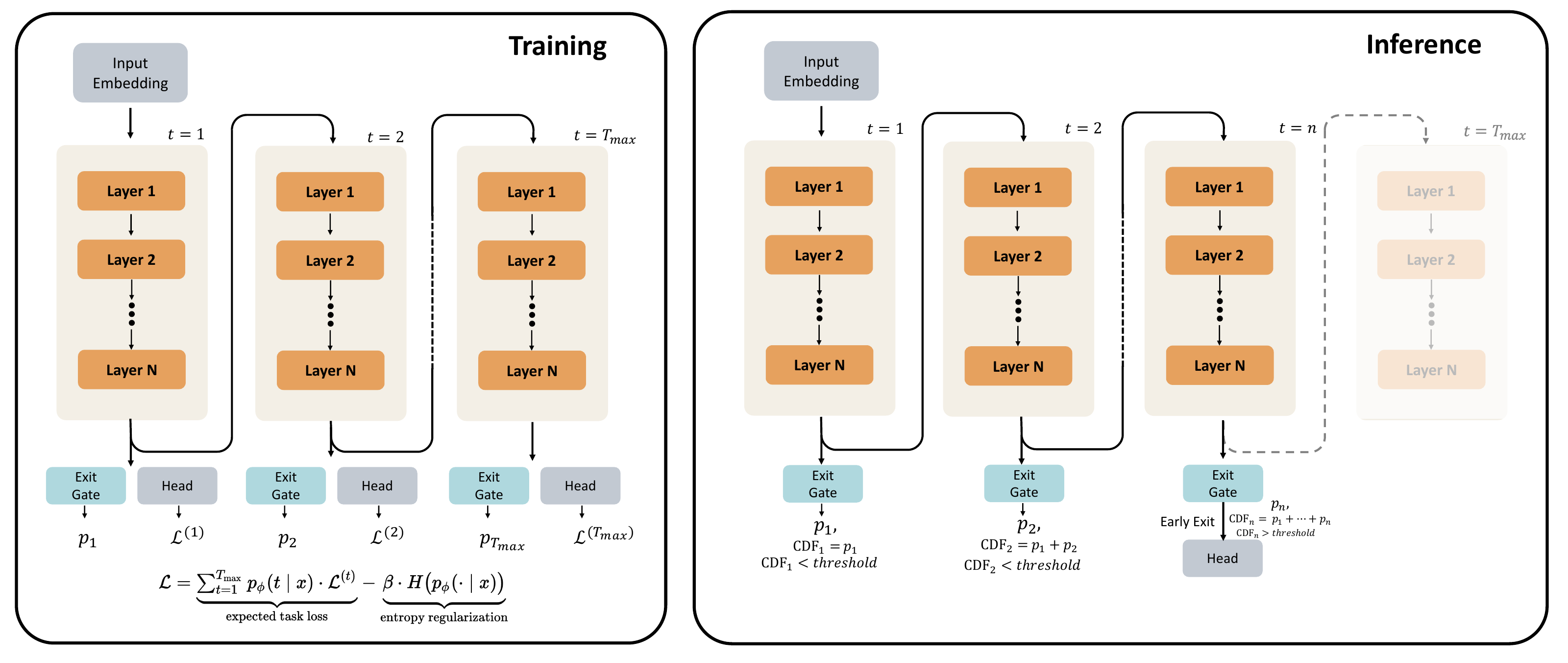
1. Predict at every loop. For token position \(i\), the representation after loop \(r\) gives a next-token loss
All loop depths therefore have a possible readout. The training question is how much weight to assign to each one.
2. Turn exit gates into a distribution over depth. A sigmoid gate produces \(\lambda_{i,r}\), the conditional probability of exiting at loop \(r\) given that computation has reached it. Define the probability of surviving the first \(r\) loops as
The probability of first exiting at a particular depth is then
The last loop receives all remaining probability mass. Without this boundary condition, some probability would describe computation continuing beyond the permitted budget.
3. Train the model and gates jointly. Using a token-level form of the paper’s objective, with \(\mathcal V\) the valid prediction positions,
The first term is an expected prediction loss. The second is negative entropy, so minimizing it encourages the gate distribution to retain several possible exit depths instead of prematurely concentrating on one. Equivalently, it is a KL penalty toward a uniform depth prior, up to an additive constant. It does not itself impose a preference for the shortest computation. LoopLM, Sections 3.1–3.3
4. Calibrate stopping separately. The second gate-training stage freezes the language model. It measures the positive reduction in each token’s loss from loop \(r-1\) to \(r\) and converts that detached improvement into a soft continuation target. Binary cross-entropy then trains the gate to predict whether refinement is still making progress. This is a local improvement signal, not knowledge of the token’s optimal future exit depth. LoopLM, Section 3.4
At inference, Q-exit means quantile exit. Accumulate the learned exit probabilities and stop at the first depth whose cumulative mass reaches a chosen threshold \(q\):
A larger threshold permits more loops for the same gate outputs. The final depth always exits because its cumulative mass is one. This is a deterministic stopping rule over a probability distribution; the “Q” here does not denote a Q-learning action value. LoopLM, Section 3.2
Pseudocode: Shared Depth, Weighted Loss, and Exit
The following PyTorch-style sketch is a pedagogical token-level realization of the joint objective. tokens and targets are already shifted for next-token prediction, both with shape [B, L]; the boolean mask valid selects supervised positions. shared_stack includes causal masking and position handling, and the same instance is called at every loop. Training evaluates all candidate depths to form the expected loss.
import torch
import torch.nn.functional as F


def looplm_joint_loss(model, tokens, targets, valid, loops, beta):
    assert loops >= 1 and valid.any()
    targets = targets.masked_fill(~valid, -100)
    h = model.embed(tokens)
    survival = torch.ones_like(tokens, dtype=torch.float32)
    objective = torch.zeros_like(survival)

    for r in range(1, loops + 1):
        h = model.shared_stack(h)              # Reuse the same weights.
        logits = model.lm_head(h)              # [B, L, vocabulary]
        ce = F.cross_entropy(
            logits.transpose(1, 2), targets, reduction="none"
        )                                     # [B, L]

        if r == loops:
            exit_mass = survival              # Force the final exit.
        else:
            hazard = model.exit_gate(h).squeeze(-1).sigmoid()
            exit_mass = survival * hazard
            survival = survival * (1.0 - hazard)

        negative_entropy = exit_mass * exit_mass.clamp_min(1e-8).log()
        objective = objective + exit_mass * ce + beta * negative_entropy

    return objective[valid].mean()


def quantile_exit(exit_masses, q):
    # One token's normalized distribution, including final residual mass.
    cumulative = 0.0
    for depth, mass in enumerate(exit_masses, start=1):
        cumulative += mass
        if cumulative >= q:
            return depth
    return len(exit_masses)                    # Floating-point safeguard.
For example, conditional exit probabilities of 0.2, 0.5, and 0.5, followed by a forced fourth exit, give masses [0.2, 0.4, 0.2, 0.2]. Threshold \(q=0.5\) exits at depth 2; \(q=0.9\) exits at depth 4. A real decoder accumulates these masses as it runs and can stop before evaluating later loops; quantile_exit isolates the decision rule for inspection. Per-token exit decisions still need an execution policy for attention, batching, and caches. The sketch omits that policy and the separate gate-calibration stage.
TRM and LoopLM: Shared Principle, Different Algorithms
At the level of state transitions, both reuse a learned computation:
Here \(\mathcal R_\theta\) is the complete TRM cycle defined earlier: \(n\) updates to \(z\) followed by one update to \(y\), all using the same \(f_\theta\). Thus one TRM cycle contains several network calls; it is not equivalent to one pass through LoopLM’s stack.
| Design choice | TRM in Less is More | LoopLM / Ouro |
|---|---|---|
| Prediction task | Supervised structured input–solution pairs; output positions predicted in parallel | Autoregressive next-token prediction on language-model corpora |
| Persistent state | Answer representation \(y\) and auxiliary reasoning state \(z\) | Hidden representation \(h\) at each token position |
| Reused module | A tiny network, typically two layers; non-causal self-attention or token-mixing MLP | A causal Transformer stack: 24 layers for Ouro-1.4B, 48 for Ouro-2.6B |
| Input conditioning | Embedded question \(x\) is added during each reasoning-state update | Token embeddings initialize the recurrence in the paper’s formulation |
| Supervision | Answer loss after each supervision step, plus a correctness-based halt loss | Next-token losses across loop depths, weighted by learned exit probabilities, plus entropy regularization |
| Gradient schedule | First \(T-1\) complete cycles without gradients; final cycle tracked; carried states detached between supervision steps | Joint loop-weighted objective, then a separate stage that freezes the LM and trains gates |
| Halting in the reported setup | Learned early halting during training; full supervision-step budget at evaluation | Quantile-based early exit explicitly studied at inference |
Sources: TRM, Section 4 and algorithm, official TRM implementation, and LoopLM, Sections 3–4. LoopLM’s method description does not prescribe TRM’s no-gradient-prefix schedule; the shared architectural idea should not be taken to imply an identical backward pass.
The most precise description is that attention-based TRM belongs to the broader recurrent-depth Transformer family, with a specialized two-state update and supervision scheme. Its MLP variant retains the recurrence but removes the Transformer attention mechanism. This is an architectural connection: LoopLM’s related-work discussion places Ouro among earlier looped and recurrent-depth models and does not identify TRM as its precursor.
TRM Implementation
Data preparation
Before following the recursive computation, we need to define what one training example contains. In the original puzzle implementation, the input is a grid and the target is its completed or transformed grid. The model predicts the output positions in parallel. The ground-truth output supplies supervision; it is not the initial answer state \(y\) fed into the recursion.
1. Convert grids into fixed-length token sequences
The official builders use small task-specific vocabularies and flatten grids in row-major order:
| Dataset | Sequence length | Token conventions |
|---|---|---|
| Sudoku | \(9\times9=81\) |
0: padding; 1: empty cell; 2–10: digits 1–9 |
| ARC | \(30\times30=900\) |
0: padding; 1: grid boundary (<eos>); 2–11: colors 0–9 |
For Sudoku, the builder reads the incomplete board and its solution from the source CSV, converts . to zero, then adds one to every cell. A raw row beginning [0, 5, 0] becomes [1, 6, 1]. The label contains the full solved board, including the positions already given in the input. Consequently, an empty input cell is a valid token, not a position to ignore in the loss. Sudoku builder
ARC inputs and outputs may have different dimensions. Each grid is placed on a separate \(30\times30\) canvas. The builder adds a row of boundary tokens immediately below the grid and a column immediately to its right, wherever the canvas has space. This <eos> is a spatial boundary, rather than a single token appended to a sentence. Original black pixels become token 2, so they remain distinguishable from padding. Training translations move an input/output pair by the same offset. ARC encoding
2. Keep examples, puzzle identities, and augmentation groups separate
Each split saves all__inputs.npy, all__labels.npy, all__puzzle_identifiers.npy, all__puzzle_indices.npy, and all__group_indices.npy, together with dataset.json. The two offset arrays describe this hierarchy:
original puzzle / group
  └── original version and augmented versions
        └── input/output examples belonging to each version
A Sudoku version has one example and always uses identifier 0. An ARC version can contain several examples and receives its own nonzero identifier. Its demonstrations and held-out queries share that identifier across splits. The model uses this ID to look up a trainable puzzle embedding. Each demonstration is stored as an individual input/output pair; the builder does not concatenate all demonstrations into a textual prompt. The loader expands the stored identifier to one ID per selected example. ARC serialization, input embeddings
3. Augment without mixing supervision across splits
Sudoku subsampling happens on the original training boards before augmentation. Each transformation is applied identically to the board and solution: relabel digits, optionally transpose, and permute rows within bands, columns within stacks, and the bands/stacks themselves. The documented --subsample-size 1000 --num-aug 1000 retains 1,000 original boards, each with its original version plus 1,000 transformed versions. The test boards receive no augmentation. Sudoku augmentation
For ARC, a rotation/reflection and color permutation are shared across every example of a task; black stays black. Duplicate transformed tasks are filtered, so the requested augmentation count is an upper bound. Spatial/color variants are built for both splits; translation is enabled only for training, with one example per version kept at the top-left origin. ARC augmentation
The ARC split deserves care: demonstrations from evaluation tasks deliberately enter training, while their query outputs go to the test split. This is a protocol with access to each evaluation task’s demonstrations, not an unseen-task holdout. Keep query answers out of training labels when reproducing it. The builder substitutes [[0]] when solutions are missing; those placeholders cannot support accuracy measurements. The README also warns that ARC-2 training contains some ARC-1 evaluation tasks, so combining the two training sets compromises an ARC-1 evaluation. Split routing, dataset instructions
4. Construct a batch and preserve its labels through recursion
The loader shuffles original groups, samples one version per visited group, and packs that version’s examples into a global batch. It samples only as many examples as the remaining capacity permits, then partitions the batch across devices. Training drops an incomplete final batch; evaluation pads it. Thus, one group traversal does not enumerate every stored augmentation. Batch sampling
The following simplified pseudocode shows the encoding and batch contract; split routing, augmentation selection, and distributed sampling are omitted:
import numpy as np
import torch

def encode_sudoku(grid):
    return np.asarray(grid, dtype=np.int32).reshape(81) + 1

def encode_arc(grid, offset=(0, 0)):
    grid = np.asarray(grid, dtype=np.int32)
    h, w = grid.shape
    r, c = offset  # Use the same valid offset for input and output.
    assert r >= 0 and c >= 0 and r + h <= 30 and c + w <= 30
    canvas = np.zeros((30, 30), dtype=np.int32)
    canvas[r:r+h, c:c+w] = grid + 2
    if r + h < 30:
        canvas[r+h, c:c+w] = 1
    if c + w < 30:
        canvas[r:r+h, c+w] = 1
    return canvas.reshape(900)

def collate(encoded_inputs, encoded_outputs, puzzle_ids):
    inputs = np.stack(encoded_inputs).astype(np.int32)
    labels = np.stack(encoded_outputs).astype(np.int32)
    labels[labels == 0] = -100  # Ignore output padding only.
    return {
        "inputs": torch.from_numpy(inputs),       # [B, L]
        "labels": torch.from_numpy(labels),       # [B, L]
        "puzzle_identifiers": torch.tensor(puzzle_ids, dtype=torch.int32),
    }                                             # IDs: [B]
The actual key is labels. The loss excludes -100, averages over valid positions per example, and supervises ARC boundary tokens as well as colors. Labels are retained in carry.current_data: only previously halted slots accept new examples and reset their states; unfinished slots keep their existing inputs, identifiers, and labels. The loss reads these retained labels, ensuring supervision stays aligned with the puzzle being refined. Collation, carry update, loss
The relation-extraction adaptation later in this post changes this contract: it tokenizes text and supervises an answer position. Its vocabulary, sequence length, and label mask must therefore be designed for that task; the original grid encodings do not establish its performance.
Main process

The model is fascinating and quite complex. It’s a recursive reasoning architecture with adaptive computation time (ACT), two interacting hidden states \(z_L\) and \(z_H\) and halting logic via Q-learning.
Data Flow
The model maintains two levels of latent states:
- \(z_H\): High-level state with shape
[batch_size, seq_len + puzzle_emb_len, hidden_size](i.e., the output \(y\) in this paper) - \(z_L\): Low-level state with the same shape as \(z_H\) (i.e., the output \(z\) in this paper)
┌─────────────────────────────────────────────────────────────┐
│                        Forward Pass                          │
└─────────────────────────────────────────────────────────────┘

Input: batch = {inputs, puzzle_identifiers, targets}
       carry = {z_H, z_L, steps, halted, current_data}

                         ↓
           ┌─────────────────────────┐
           │  Reset carry if halted  │
           │  z_H = H_init           │
           │  z_L = L_init           │
           └─────────────────────────┘
                         ↓
           ┌─────────────────────────┐
           │  Input Embeddings       │
           │  tokens + puzzle + pos  │
           └─────────────────────────┘
                         ↓
           ┌─────────────────────────────────────┐
           │  Recursive Reasoning (no grad)      │
           │  ┌─────────────────────────────┐    │
           │  │ For h in range(H_cycles-1): │    │
           │  │   For l in range(L_cycles): │    │
           │  │     z_L ← L(z_L, z_H + x)   │    │
           │  │   z_H ← L(z_H, z_L)         │    │
           │  └─────────────────────────────┘    │
           └─────────────────────────────────────┘
                         ↓
           ┌─────────────────────────────────────┐
           │  Final Reasoning Cycle (with grad)  │
           │  For l in range(L_cycles):          │
           │    z_L ← L(z_L, z_H + x)            │
           │  z_H ← L(z_H, z_L)                  │
           └─────────────────────────────────────┘
                         ↓
           ┌─────────────────────────┐
           │  Output Generation      │
           │  logits = lm_head(z_H)  │
           │  q_halt = q_head(z_H₀)  │
           └─────────────────────────┘
                         ↓
           ┌─────────────────────────┐
           │  Halting Decision       │
           │  (ACT mechanism)        │
           └─────────────────────────┘
                         ↓
Output: new_carry = {z_H', z_L', steps+1, halted', current_data}
        outputs = {logits, q_halt_logits, q_continue_logits}
Q-Learning
Q-Learning is a reinforcement learning algorithm that learns to make decisions by estimating the quality Q-value of taking specific actions in specific states.
More specifically, if \(Q(state, action)\) is the expected future reward for taking action in state, then the Q-value of the optimal policy can be iteratively updated by the following Bellman equation:
\(Q(s, a) = Q(s, a) + \alpha [r + \gamma \max_{a'} Q(s', a') - Q(s, a)]\) where \(r\) is the reward for taking action \(a\) in state \(s\), \(\gamma\) is the discount factor, \(\alpha\) is the learning rate, \(s'\) is the next state, and \(a'\) is the next action.
The Q-value of the optimal policy is the maximum Q-value of all possible actions in all possible states.
\[Q^*(s, a) = \max_{a'} Q(s, a')\]Q-Learning in TRM
In TRM, the Q-learning is used to learn the halting policy, i.e., when to stop the reasoning process. More specifically, there are two actions need to be considered:
- Halt: Stop reasoning and return the output answer.
- Continue: perform one more reasoning cycle.
In the implementation, the Q-value is the output of the q_head of the model.
self.q_head = CastedLinear(self.config.hidden_size, 2, bias=True) # 2 actions: halt and continue
q_logits = self.q_head(z_H[:, 0]) # Using the first token of the high-level state as the state representation
q_halt_logits = q_logits[:, 0] # Q(state, halt)
q_continue_logits = q_logits[:, 1] # Q(state, continue)
The halting logic is implemented as follows:
if self.config.no_ACT_continue:
    halted = (q_halt_logits > 0) # Halt if Q(halt) is positive
else:
    halted = (q_halt_logits > q_continue_logits) # Halt if Q(halt) is greater than Q(continue)
Q-Learning Loss
The Q-learning loss is defined in the ACTLossHead class as below:
q_halt_loss = F.binary_cross_entropy_with_logits(
    outputs["q_halt_logits"],        # Predicted: should we halt?
    seq_is_correct.to(...),          # Target: 1 if sequence is correct, 0 otherwise
    reduction="sum"
)
Where seq_is_correct is the target for the Q-learning loss, 1 if the model’s prediction is completely correct (all tokens match), 0 otherwise.
As noted, seq_is_correct is binary, either all tokens are correct or the sequence is wrong.
# Token-level correctness
mask = (labels != IGNORE_LABEL_ID)  # Valid positions
is_correct = mask & (torch.argmax(outputs["logits"], dim=-1) == labels)

# Sequence-level correctness (ALL tokens must be correct)
loss_counts = mask.sum(-1)  # Number of valid tokens per sequence
seq_is_correct = is_correct.sum(-1) == loss_counts  # Boolean: all tokens correct?
Continue Loss
In addition, the authors also proposed to use the Q-Continue Loss (bootstrapped Q-values) (The question Should we continue? instead of Should we halt?).
However, as noted by the authors, while the Q-continue loss fits Q-learning, but seems totally unnecessary as the Q-halt loss is enough to learn the halting policy.
if "target_q_continue" in outputs:
    q_continue_loss = F.binary_cross_entropy_with_logits(
        outputs["q_continue_logits"],  # Predicted: should we continue?
        outputs["target_q_continue"],  # Target: bootstrapped Q-value from next state
        reduction="sum"
    )
where target_q_continue is the bootstrapped Q-value from the next state.
target_q_continue = sigmoid(max(next_q_halt, next_q_continue))
Total loss
total_loss = lm_loss + 0.5 * (q_halt_loss + q_continue_loss)
where lm_loss is the standard cross-entropy on token predictions.
Training Dynamics of Q-Learning
Early phase: Init Q-head
The Q-head is initialized to (almost) zero for faster learning during bootstrapping, i.e., never halts early (always uses max steps). This forces the model to learn basic language understanding before adapting to the reasoning task.
# Q head special init
# Init Q to (almost) zero for faster learning during bootstrapping
with torch.no_grad():
    self.q_head.weight.zero_()
    self.q_head.bias.fill_(-5)  # type: ignore
Phase 2: Learning to halt
As language understanding improves, seq_is_correct becomes more frequent and reliable, Q-head starts to learn correlation between reasoning state and correctness,
resulting in the model learning to halt early.
Phase 3: Exploration Refinement
# Force trying different step counts
min_halt_steps = random_int(2, halt_max_steps) with probability ε
The model exploration prevents the model always halts at the same step, thus leading to overfitting. This helps to discover optimal reasoning depth for different problems.
Applying to Relation Extraction problem
Relation Extraction (RE)
Relation Extraction (RE) is a core task in Natural Language Processing (NLP) that involves identifying and classifying semantic relationships between entities mentioned in text.
For example, given the sentence "John Smith is a patient of Dr. Emily Johnson", an RE system should detect the relationship between John Smith and Dr. Emily Johnson as "patient of".
Similarly, in the sentence "Aspirin is used to treat headache", the identified relationship is "used to treat" between two entities Aspirin and headache.
The set of possible relationships is typically predefined and fixed for a given task.
Importantly, the label "no relation" is also a valid category, indicating that no meaningful semantic link exists between the mentioned entities.
Traditional approaches to RE include rule-based methods, feature-based classifiers, and neural architectures leveraging contextual embeddings such as BERT. Recent advances, however, have explored formulating RE as a question answering (QA) problem, giving rise to methods such as QA4RE.
BioRED Dataset
The dataset used in this demo is the BioRED dataset. BioRED is a first-of-its-kind biomedical RE corpus with multiple entity types (e.g., gene/protein, disease, chemical) and relation pairs (e.g., gene-disease; chemical-chemical) at the document level, on a set of 600 PubMed abstracts. The data, pretrained models (for the RE task) and annotation guidelines are provided in the link: https://ftp.ncbi.nlm.nih.gov/pub/lu/BioRED/.
Data Format
The BioRED dataset adopts the PubTator format, a structured, plain-text representation commonly used for biomedical text annotations. Each document—typically a PubMed abstract—contains both text and text-bound annotations describing entities and relations. The format includes the following components:
- PMID: The PubMed identifier, followed by the document title and abstract text.
-
Entity annotations: Each entity is represented as
PMID \t start-index \t end-index \t text-span \t entity_type \t normalized_id. -
Relation annotations: Each relation is encoded as
PMID \t relation-type \t normalized_id1 \t normalized_id2 \t novelty.
An example of the PubTator-formatted document is shown below:
Example of PubTator-formatted document

15485686|t|A novel SCN5A mutation manifests as a ...

15485686|a|OBJECTIVE: Congenital long QT syndrome (LQTS) ...

15485686 8 13 SCN5A GeneOrGeneProduct 6331

15485686 56 72 long QT syndrome DiseaseOrPhenotypicFeature D008133

15485686 Association D001919 6331 Novel

15485686 Positive_Correlation D001919 p|SUB|V|1763|M Novel
Each document \(S\) may contain multiple entities \(E_i\) and relations \(R_{ij}\) between them. Importantly, no entity pair \((E_i, E_j)\) has more than one relation in the dataset—each pair is associated with at most a single relation \(R_{ij}\).
Thus, the task in BioRED can be defined as: given a document \(S\) and a set of entities \(E\), extract all relations \(R_{ij}\) that hold between entity pairs \((E_i, E_j)\) within the text.
Entity Types
BioRED defines six entity types (five major biomedical categories and one infrequent type, Cell Line), each normalized to an external biomedical knowledge base. The entity taxonomy is summarized in the table below.
| Entity Type | Examples | Normalization Source |
|---|---|---|
| Gene (Protein) | ABCA1, CYP2D6, BMP | NCBI Gene |
| Variant (Residue) | S276T, rs2234671, c.435C>G | dbSNP |
| Species | Homo sapiens, E. coli | NCBI Taxonomy |
| Disease (Symptom) | Hypertension, Alzheimer’s disease | MEDIC (MeSH + OMIM) |
| Chemical | Terbutaline, Acetaminophen | MeSH: Chemicals and Drugs |
| Cell Line | MCF7/AdrR | Cellosaurus |
Entity types in BioRED and their corresponding normalization sources.
Relation Types
BioRED defines a comprehensive set of pairwise relations between concept types. Each relation is explicitly typed—either directional or non-directional—and falls into one of three major semantic categories: Positive Correlation, Negative Correlation, or Association. In addition to these, several specialized relation types capture more specific biomedical interactions, including Bind, Co-treatment, Comparison, Drug Interaction, and Conversion.
During dataset preprocessing, a special category labeled None is added to represent negative examples, denoting entity pairs with no annotated relationship.

Data Processing
In order to apply the TRM to the RE task, we need to convert the BioRED dataset into the format that can be used by the TRM. However, there are three main challenges making it is not straightforward:
- Variable Text Length. The current TRM expects a fixed length input (i.e., for the Sudoku puzzle, the input is a 9x9 grid), but biomedical texts vary greatly in length. We need to set a larger sequence length and truncate/padding the texts if necessary.
- Classification vs Generation task. The TRM is designed for the generation task, while the original RE task is a classification task. One of the approaches can be used is to convert the RE task into a multiple-choice generation task, where the model needs to generate the relation type options for the given entity pairs.
- Entity awareness. Unlike the Sudoku puzzle, the input in RE task contains the full text of the document and the entity pairs. In the dataset, one document may contain multiple entity pairs with multiple relations between them. Therefore, in order to answer specific relation type for a specific entity pair, the model needs to be aware of that entity pair, distinguish it from other entity pairs. Some potential solutions can be: adding special marker tokens around entities, use entity type embedding or create position-aware prompts. In this demon, we use the simplest solution, that is, adding special marker tokens around entities and move the two entities to the beginning of the input sequence.
The input format is shown below:
Input sequence:
[CLS] <E1> entity1_text </E1> [SEP] <E2> entity2_text </E2> [SEP]
full_text [SEP]
Options: A) Association B) PositiveCorrelation C) ... [SEP]

Label sequence:
[-100, -100, ..., -100, A, -100, -100, ...]
                        ↑
                   Only supervise answer token
References
[1] Jolicoeur-Martineau, Alexia. “Less is More: Recursive Reasoning with Tiny Networks.” arXiv preprint arXiv:2510.04871 (2025).
[2] Luo, Ling, et al. “BioRED: a rich biomedical relation extraction dataset.” Briefings in Bioinformatics 23.5 (2022): bbac282.
Enjoy Reading This Article?
Here are some more articles you might like to read next: