Comprehensive Algorithm Portfolio Evaluation using Item Response Theory
About the paper
- Link to the paper: https://arxiv.org/abs/2307.15850
- Authors: Sevvandi Kandanaarachchi, Kate Smith-Miles, CSIRO, Uni Melb
- Talk at OPTIMA ARC and its slide
Summary
The paper proposed a framework to evaluate a portfolio of algorithms using Item Response Theory (IRT). Instead of using the standard IRT mapping, the authors proposed to invert the mapping by considering the datasets as agents and the algorithms as items. By using this mapping, the IRT model now can give more insights about the characteristics of algorithms including the algorithm anomalousness, consistency, and dataset difficulty. In addition, the framework also provides analysis of strengths and weaknesses of algorithms in the problem space which can be used to select the best algorithm for a given dataset.
Item Response Theory
Item Response Theory (IRT) is a psychometric theory that models the relationship between the latent trait (such as verbal or mathematical ability, that cannot be directly measured) of a person and the probability of a person to answer a question correctly. Using the participant responses to the test items, an IRT model is fitted to estimate the discrimination and difficulty of test items and the ability of participants.
Family of IRT models
Dichotomous IRT model
The simplest IRT model is the dichotomous IRT model, which assumes that the probability of a person to answer a question correctly is a logistic function of the difference between the person’s ability and the item’s difficulty. The model is formulated as follows:
\[P(X_{ij} = 1 \mid \theta_i, \alpha_j, \beta_j) = \frac{1}{1 + e^{- \alpha_j (\theta_i - \beta_j)}}\]where \(X_{ij}\) is the response of person \(i\) to item \(j\), \(\theta_i\) is the ability of person \(i\), \(\beta_j\) is the difficulty of item \(j\), and \(\alpha_j\) is the discrimination parameter.
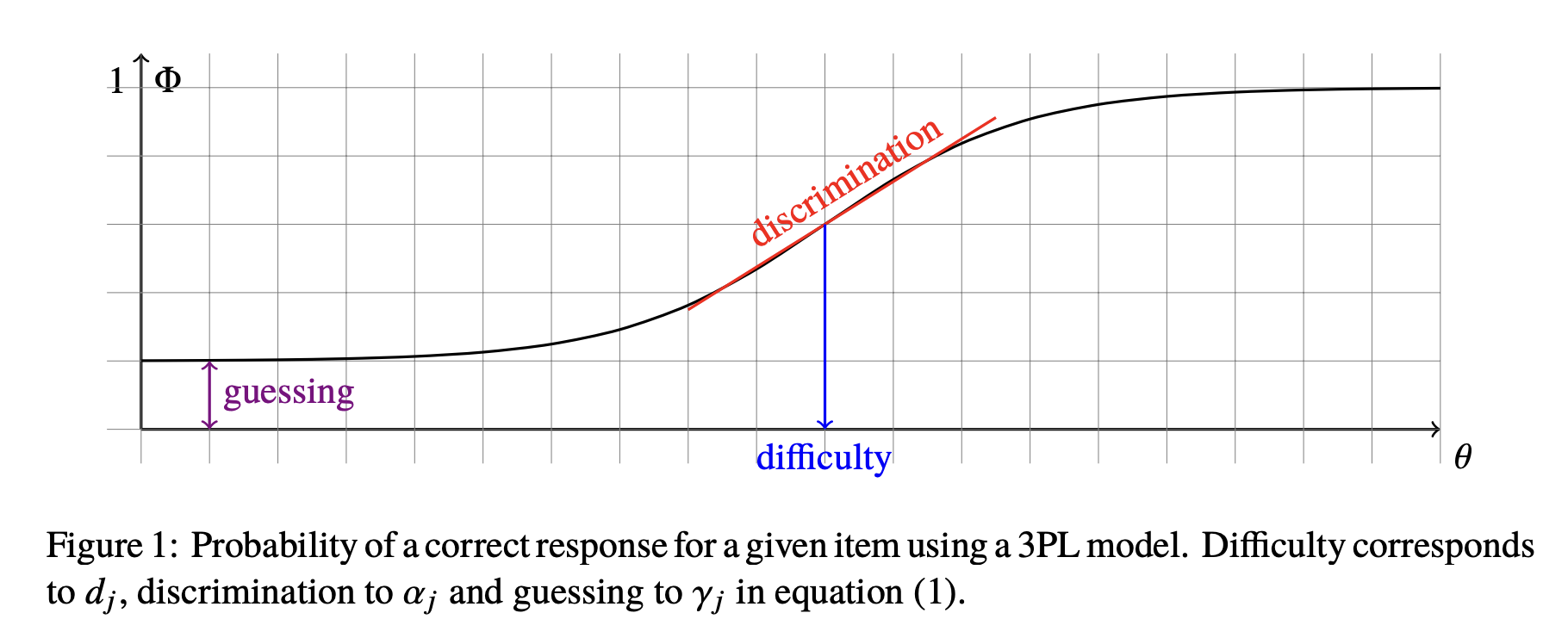
3PL: introducing one additional guesing parameter \(\gamma_j\) to the model:
\[P(X_{ij} = 1 \mid \theta_i, \alpha_j, \beta_j, \gamma_j) = \gamma_j + (1 - \gamma_j) \frac{1}{1 + e^{- \alpha_j (\theta_i - \beta_j)}}\]Figure below shows the probability of a person to answer a question correctly as a function of the person’s ability \(\theta_i\) given the item’s parameters \(\alpha_j, \beta_j, \gamma_j\).
Polytomous IRT model
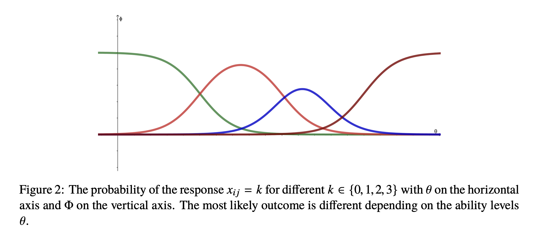
The polytomous IRT model is an extension of the dichotomous IRT model that allows for more than two response categories (e.g., an answer is marked not just correct/incorrect but with score from 1 to K). The most common polytomous IRT model is the graded response model (GRM), in which the cummulative probabilities of a person to get a higher or equal to score \(k\) is formulated as follows:
\[P(X_{ij} \geq k \mid \theta_i, \alpha_j, \beta_j^k) = \frac{1}{1 + e^{- \alpha_j (\theta_i - \beta_j^k)}}\]where \(X_{ij}\) is the response of person \(i\) to item \(j\), \(\theta_i\) is the ability of person \(i\), \(\beta_j^k\) is the difficulty of item \(j\) for response category \(k\), and \(\alpha_j\) is the discrimination parameter. Each item \(j\) has a set of difficulties \(\beta_j = \{ \beta_j^k \}_{k=1}^K\) which is making sense because the difficulty of an item is different for different response categories.
The probability of a person to get a score \(k\) is formulated as follows:
\[P(X_{ij} = k \mid \theta_i, \alpha_j, \beta_j) = P(X_{ij} \geq k \mid \theta_i, \alpha_j, \beta_j^k) - P(X_{ij} \geq k+1 \mid \theta_i, \alpha_j, \beta_j^{k+1})\]Given parameters \(\alpha_j, \beta_j\) are known and fixed, the probability of a person to get a score \(k\) is a curve that is a function of the person’s ability \(\theta_i\). And given the person’s ability \(\theta_i\) and the item’s parameters \(\alpha_j, \beta_j\), we can estimate the most likely score \(k\) of the person which is the score that maximizes the probability \(P(X_{ij} = k \mid \theta_i, \alpha_j, \beta_j)\).
Continuous IRT model
The continuous IRT model is an extension of the dichotomous IRT model that allows for continuous responses (e.g., the response is a real number between 0 and 1). The density function of the continuous IRT model is formulated as follows:
\[f(z_{ij} \mid \theta_i) = \frac{\alpha_j \gamma_j}{2 \pi} \exp(- \frac{\alpha_j^2}{2}(\theta_i - \beta_j - \gamma_j z_j))\]where \(\theta_i\) is the ability of person \(i\), \(\beta_j\) is the difficulty of item \(j\), \(\alpha_j\) is the discrimination parameter, and \(\gamma_j\) is the scaling factor. \(z_{ij}\) is the normalized response of person \(i\) to item \(j\) which is formulated as follows:
\[z_{j} = \ln \frac{x_{j}}{ k_j - x_j}\]where \(x_{j}\) is a continuous score between 0 and \(k_j\) and \(k_j\) is the maximum score of item \(j\). \(z_j\) has a range between \(-\infty\) and \(\infty\).
In this model, these are total 3 parameters for each item \(j\) (i.e., \(\beta_j, \alpha_j, \gamma_j\)$) and 1 parameter for each person \(i\) (i.e., \(\theta_i\)$). Unlike the polytomous IRT model, the difficulty \(\beta_j\) of an item \(j\) is the same for all response categories.
Mapping algorithm evaluation to IRT
To understand the mapping better, let’s consider the following components of IRT:
- The agents: a group of students or algorithms in which each agent is associated with a set of characteristics (e.g., ability of a student, parameters of an algorithm)
- The items: a set of questions or datasets in which each item is associated with a set of characteristics (e.g., difficulty, discrimination, bias)
- The responses: the responses of agents to items (e.g., the responses of students to questions, the performance of algorithms on datasets)
IRT models the relationship between the characteristics of agents and items and the responses of agents to items. The goal of IRT is to estimate the characteristics of agents and items given the responses of agents to items, with the primary goal of estimating the characteristics of items (e.g., the difficulty of questions which is broader interest than the ability of each individual student).
It can be seen that, in the dichotomous IRT model, there are two parameters of an item (i.e., difficulty and discrimination) and one parameter of an agent (i.e., ability). In the polytomous IRT model, for each item, there are \(K\) parameters of difficulty (i.e., \(\{\beta_j^k\}_{k=1}^K\)$) and one parameter \(\alpha_j\) for discrimination, while there is only one parameter of an agent (i.e., ability \(\theta_i\)$).
Mapping algorithm evaluation to IRT:
In the context of algorithm evaluation, the agents are algorithms and the items are datasets. The responses are the performance of algorithms on datasets. Let \(f_{\theta_i}\) is an agent (i.e., an algorithm) parameterized by \(\theta_i\). \(x_j\) is an item (i.e., a dataset) belonging to set of items \(X\), each dataset \(x_j\) is associated with a set of characteristics \(c_j\) (e.g., difficulty, discrimination, bias).
Within the context, the IRT model now estimates the probability of an algorithm \(f_{\theta_i}\) to solve a dataset \(x_j\) given the characteristics \(c_j\) of the dataset and the ability \(\theta_i\) of the algorithm.
However, as the authors mentioned in the paper, with this standard mapping, the IRT model is focusing on evaluating the characteristics of datasets (i.e., items) rather than the characteristics of algorithms (i.e., agents). Therefore, the authors proposed to invert the mapping by considering the datasets as agents and the algorithms as items.
By using the inverted mapping, the IRT model now can give more insights about the characteristics of algorithms rather than the characteristics of datasets, thanks to the fact that there are more parameters to be estimated for each algorithm (i.e., 3 parameters for each algorithm in the continuous IRT model) than for each dataset (i.e., 1 parameter for each dataset in the continuous IRT model).
More specifically, if we consider the continuous IRT model and the inverted mapping, the following are the parameters of the model:
- \(\beta_j\) is the difficulty of item \(j\), in this case, the (reversed) difficulty limit of algorithm \(j\).
- \(\alpha_j\) is the discrimination parameter of item \(j\), in this case, the (reversed) algorithm anomalousness and consistency.
- \(\gamma_j\) is the scaling factor of item \(j\), in this case, the algorithm bias (I am not sure about this because it was not mentioned in the paper).
- \(\theta_i\) is the ability of agent \(i\), in this case, the (reversed) dataset difficulty.
Characteristics of algorithms estimated by IRT model
-
Dataset difficulty: It is estimated by \(\delta_i = -\theta_i\) which is the ability of agent \(i\), in this case the dataset difficulty. Given a fixed algorithm’s characteristics, the probability of a dataset to be solved by the algorithm will increase as \(\theta_i\) increases. Therefore, an dataset \(i\) is considered to be easy if \(\theta_i\) is large or vice versa.
-
Algorithm anomalousness: It is estimated by \(sign(\alpha_j)\) (i.e., TRUE if \(\alpha_j < 0\) and FALSE if \(\alpha_j > 0\)$) show whether the algorithm is anomalous or not. It is because in the logistic function, if \(\alpha_j < 0\), then the probability of the agent (i.e., a dataset) act on the item (i.e., an algorithm) is decreasing as the ability of the agent increases (i.e., \(\theta_i\) or easiness of a dataset). In other words, the algorithm is more likely to fail on a easy dataset than on a hard dataset which is an anomalous behavior.
-
Algorithm consistency: It is estimated by \(1/\|\alpha_j\|\) (i.e., inverse of the absolute value of \(\alpha_j\)$), which shows the consistency of the algorithm. It is because in the logistic function, the \(\alpha_j\) is the slope of the curve, therefore, the larger the \(\alpha_j\), the steeper the curve, which means that the algorithm is changing its behavior more rapidly as the ability of the agent changes (i.e., \(\theta_i\) or easiness of a dataset). In other words, large \(\alpha_j\) or small \(1/\|\alpha_j\|\) means that the algorithm is less consistent/stable/robust against the change of the difficulty of a dataset.
-
Difficulty limit of algorithm: It is estimated by \(-\beta_j\) which is the difficulty of item \(j\). In this case, the difficulty limit of algorithm \(j\). It is because in the logistic function, the \(\beta_j\) is the point at which the probability of the agent (i.e., a dataset) act on the item (i.e., an algorithm) is 0.5. In other words, the difficulty limit of algorithm \(j\) is the difficulty of a dataset \(i\) at which the algorithm \(j\) has 50% chance to solve the dataset \(i\). The higher difficulty limit of algorithm \(j\), the more difficult dataset that the algorithm \(j\) can solve.
-
Algorithm bias: (This was not mentioned in the paper but just my analysis) It is estimated by \(\gamma_j\) which is the scaling factor of item \(j\). In this case, the algorithm bias. It can be seen that in the continuous IRT model, the \(\gamma_j\) has to be same sign as \(\alpha_j\) (i.e., \(\alpha_j \gamma_j > 0\)$). Just consider the case when \(\gamma_j > 0\), then the higher the \(\gamma_j\), the higher the probability that the dataset is solved by the algorithm. More interestingly, the \(\gamma_j\) is the scaling factor of the response \(z_j = \ln \frac{x_j}{k_j - x_j}\) which will be very large if \(x_j\) is close to \(k_j\) (i.e., the maximum score of item \(j\)$). Therefore, the density function \(f(z_{ij} \mid \theta_i)\) will be very large if \(x_j\) is close to \(k_j\) which means that the probability of the dataset to be solved by the algorithm is very high if \(x_j\) is close to \(k_j\) which is makes sense because the dataset is easy. In contrast, the density function \(f(z_{ij} \mid \theta_i)\) will be very small if \(x_j\) is close to 0. Therefore, the continuous IRT model is strongly biased towards the extreme values of the response \(x_j\) (i.e., \(x_j = 0\) or \(x_j = k_j\)$) which is not good. However, if the scaling factor \(\gamma_j\) is small, it reduces this bias issue, vice versa. Therefore, the \(\gamma_j\) can be used to measure the bias of the algorithm.
-
Performance-Dataset Difficulty Curve: after getting all the above parameteres of \(n\) algorithms on \(N\) datasets/problems, we can estimate the performance-dataset difficulty curve \(h_j(\delta)\) of each algorithm \(j\) by using function estimation method (i.e., smoothing spline as proposed in the paper).
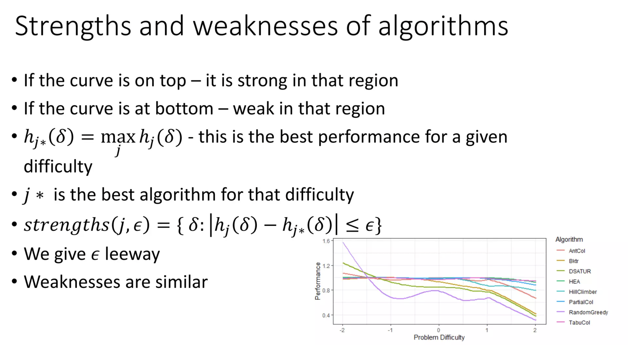
- Strengths and weaknesses of algorithm: based on the performance-dataset difficulty curve \(h_j(\delta)\), we can identify the strengths and weaknesses of each algorithm \(j\) by comparing between curves/algorithms. For example, if the curve of algorithm \(j\) is above the curve of algorithm \(k\) for all \(\delta\), then algorithm \(j\) is better than algorithm \(k\) for all \(\delta\). Given a dataset difficulty \(\delta\), we can find the best algorithm which has the highest value of \(h_j(\delta)\). We also can define a region where an algorithm can be considered as algorithm’s strengths or weaknesses.
Framework
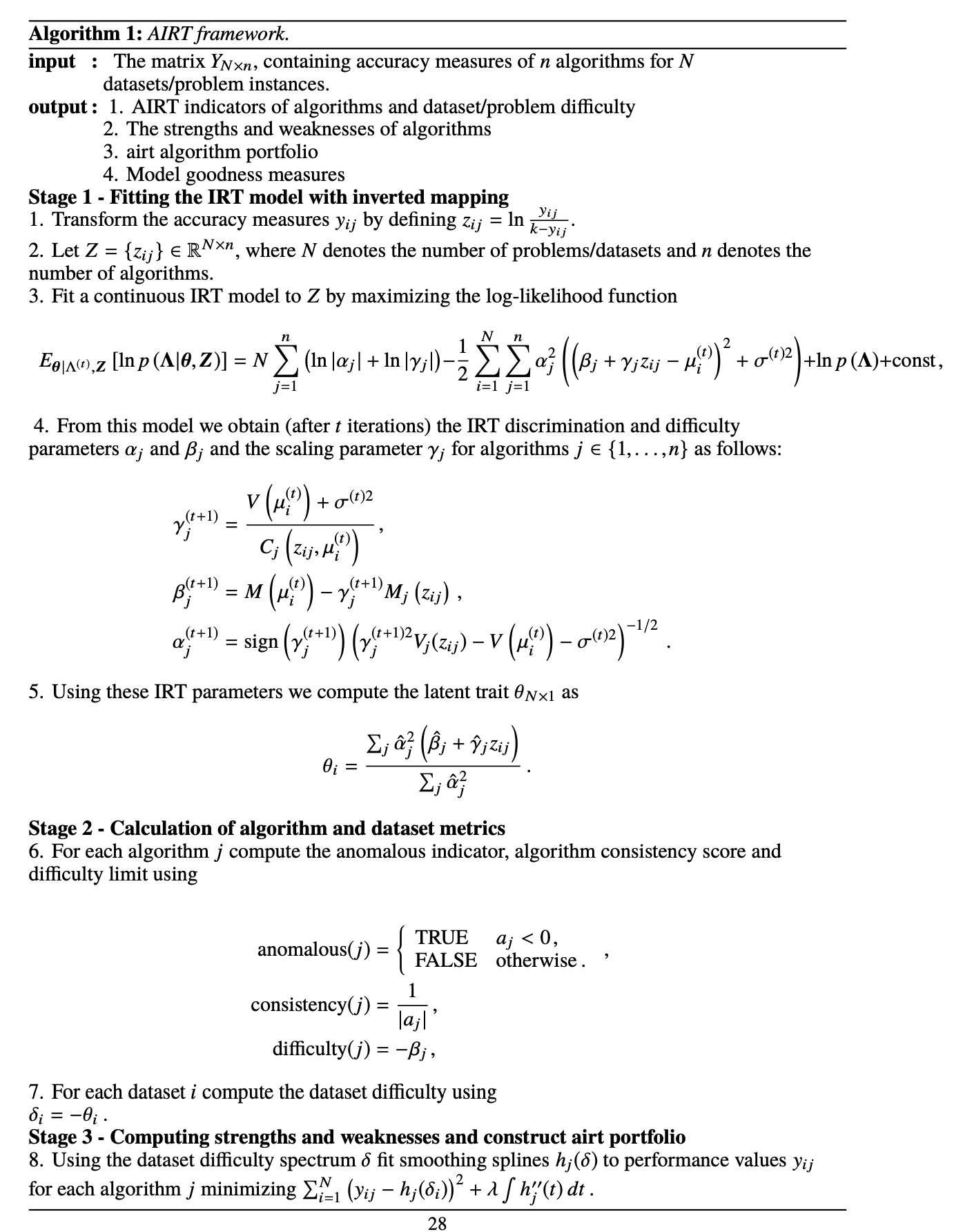
The AIRT framework can be found in page 28 of the paper, which consists of 3 main stages:
- Stage 1 - Fitting the IRT model with inverted mapping Given an input matrix \(Y_{N \times n}\) containing accuracy measures of \(n\) algorithms for \(N\) datasets, the IRT model is fitted to estimate the parameters of the model (i.e., \(\beta_j, \alpha_j, \gamma_j, \theta_i\)). The authors proposed to use the continuous IRT model with the inverted mapping. The parameters of the model are estimated using the Expectation-Maximization (EM) algorithm.
- Stage 2 - Calculation of algorithm and dataset metrics For each algorithm \(j\) compute the anomalous indicator, algorithm consistency score and difficulty limit. For each dataset \(i\) compute the dataset difficulty \(\delta_i = - \theta_i\).
- Stage 3 - Computing strengths and weaknesses and construct airt portfolio
Questions
- In IRT model, an agent (e.g., an algorithm) and an item (e.g., a dataset) are assumed to be independent. However, in the context of machine learning where an algorithm is trained on a training set and tested on a test set - which is the item in IRT model, the assumption of independence is not true. For example, a good algorithm but was trained on a biased training set will perform worse on a test set than a bad algorithm but was trained on an unbiased training set. Therefore, the performance of an algorithm on a test set is not only determined by the algorithm itself but also the training set it was trained on. So how to deal with this issue in IRT model?
- Extend the above question, how to deal with the case when many algorithms were trained on the same training set?
Future work: IRT-based Disentanglement Learning
Introduction
This project aims to disentangle ML-bias into algorithmic and data bias focussing on intersectional subgroups.
So what are algorithmic bias and data bias in the context of machine learning?
- Data bias is the bias in the training data that is used to train the ML model. It occurs when the data used for training is not representative of the real-world population or when it contains inherent biases. For example, a dataset of images of people that is used to train a facial recognition system may contain more images of white people than people of color. This can lead to the facial recognition system being less accurate when identifying people of color.
- Algorithmic bias is the bias in the algorithm itself. It occurs when the algorithm is not designed to be fair or when it is not trained to be fair. For example, a facial recognition system that is trained with purpose to identify people in a specific demographic group (e.g., white people) will be less accurate when identifying people in other demographic groups (e.g., people of color).
Recognizing data bias is a challenging task because the data bias is not always obvious and the dataset is usually large and complex. Equally complex is the task of recognizing algorithmic bias because the training process of a ML model is also complex where the bias can be introduced at any stage such as data collection, feature selection, or the choice of objective function.
To adapt the IRT model to the context of machine learning, we need to consider the following:
- The algorithm is the pretrained model which is trained on a training set (which can be biased or unbiased but we don’t know)
- The dataset is to mention the test set which is used to evaluate the algorithm. The dataset can be sampled from the same distribution as the training set or from a different distribution.
- The algorithms are assumed to be independent even are trained on the same training set. The algorithms also have the same task on the test set (e.g., the pretrained ResNet50, VGG19 models to predict an image into 1 of 10 classes).
- The dataset are assumed to be disjoint. The datasets also are served for the same task (e.g., to test performance of classification models)
- The data bias problem in this context is the bias of the test item which is used to evaluated the algorithm (not the bias of the training set as in ML literature). For example, let’s consider education system where a test item is a set of questions and an algorithm is a student. We want to evaluate diverse knowledge of students on several subjects, i.e., math, physics, chemistry, literature, etc. The data bias problem in this context is that the test item is only able to evaluate on a specific subject (e.g., math) but not on all subjects. The algorithmic bias problem in this specific example is that the student is only good at math but not good at other subjects.
Problem setting: Given \(n\) algorithms and \(N\) datasets, the goal is to identify which algorithm/dataset has bias problem. On the other words, how to distinguish a good algorithm performing poorly on a biased dataset from an equally performed bad algorithm?
Note:
- The term “disentangle learning” is commonly referred to the approach that learns disentangled representations of data in machine learning. However, in this project, the term “disentangle learning” is used to refer to the approach that disentangle ML-bias into algorithmic and data bias.
Proposed framework
We need to make some assumptions as follows:
- an biased algorithm might perform poorly on an unbiased dataset.
- an unbiased algorithm might perform poorly on a biased dataset.
- an biased algorithm might not necessary perform well on an biased dataset because it might be trained on different biased training set.
- in this project, a poor generalization algorithm which performs poorly on both biased and unbiased datasets might be different from a biased algorithm which might perform well on biased datasets but poorly on unbiased datasets.
We consider two IRT models simultaneously, the standard IRT model and the IRT model with inverted mapping. The standard IRT model is used to estimate the characteristics of datasets (i.e., difficulty, discrimination) while the IRT model with inverted mapping is used to estimate the characteristics of algorithms (i.e., difficulty limit, anomalousness, consistency).
For the IRT model with inverted mapping, we consider the performance-dataset difficulty curve \(h^d_{a_j}(\delta_d)\) of each algorithm \(a_j\), while for the standard IRT model, we consider the performance-algorithm difficulty curve \(h^a_{d_i}(\delta_a)\) of each dataset \(d_i\). With the two curves, we can identify a biased dataset as follows:
- A dataset \(d_i\) is considered to be biased if it is solved well by a biased algorithm \(a_j \in F_b\) but poorly by an unbiased algorithm \(a_j \in F_u\).
\(h^d_{a_j} (\delta_d) \leq \epsilon_{low} \; \forall \; a_j \in F_u\) \(h^d_{a_j} (\delta_d) \geq \epsilon_{up} \; \forall \; a_j \in F_b\)
- An algorithm \(a_j\) is considered to be biased if it performs well on a biased dataset \(d_i \in D_b\) but poorly on an unbiased dataset \(d_i \in D_u\).
\(h^a_{d_i} (\delta_a) \leq \epsilon_{low} \; \forall \; d_i \in D_u\) \(h^a_{d_i} (\delta_a) \geq \epsilon_{up} \; \forall \; d_i \in D_b\)
where \(\epsilon_{low}\) and \(\epsilon_{up}\) are the lower and upper thresholds, respectively.
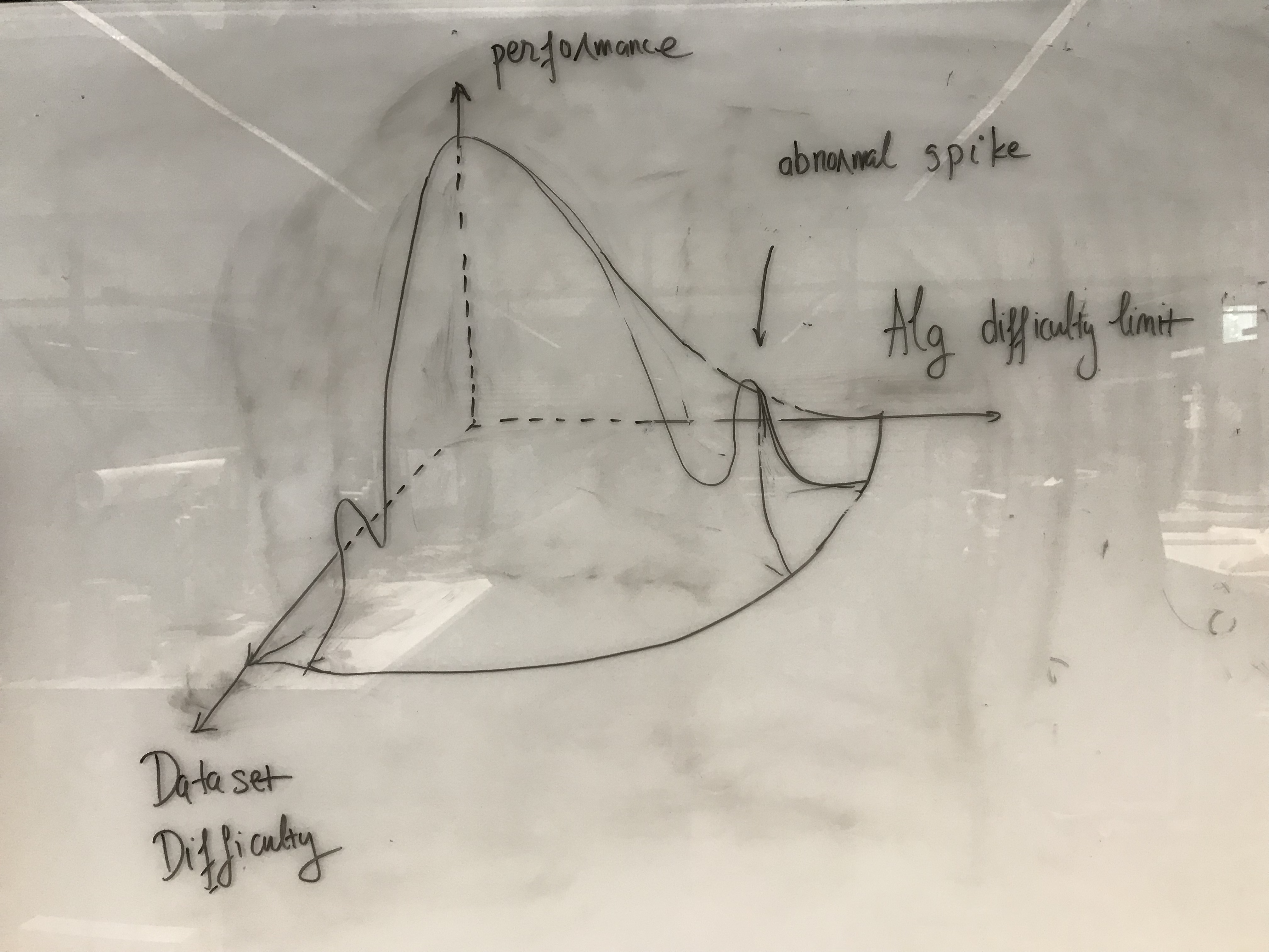
We can also a 3D map where the z-axis is the performance of an algorithm on a dataset, the x-axis is the difficulty of the dataset, and the y-axis is the difficulty limit of the algorithm.
References
Fernando Martínez-Plumed, Ricardo BC Prudêncio, Adolfo Martínez-Usó, and José HernándezOrallo. Item Response Theory in AI: Analysing machine learning classifiers at the instance level. Artificial Intelligence, 271:18–42, 2019.
Yu Chen, Ricardo BC Prudêncio, Tom Diethe, Peter Flach, et al. β3-IRT: A New Item Response Model and its Applications. arXiv preprint, arXiv:1903.04016, 2019.
Enjoy Reading This Article?
Here are some more articles you might like to read next: