Fake Taylor Swift and the Adversarial Game of Concept Erasure and Injection

How to stop generating na*ed Taylor Swift

Introduction

Recently, X (Twitter) had been flooded with sexually explicit AI-generated images of Taylor Swift, shared by many X users. As reported by The Verge, “One of the most prominent examples on X attracted more than 45 million views, 24,000 reposts, and hundreds of thousands of likes and bookmarks before the verified user who shared the images had their account suspended for violating platform policy. The post remained live on the platform for about 17 hours before its removal”. Soon after, X had to block the searches for Taylor Swift as the last resort to prevent the spread of these images (Ref to The Verge).

While this incident has certainly raised public awareness about the threat of AI-generated content, including the spread of misinformation, racism, and sexism, the general public might think such incidents only happen to famous figures like Taylor Swift and may not take it personally. However, that is not the case. With recent advancements in personalized AI-generated content, led by the Dreambooth project , it has become very easy and efficient to customize or personalize generated content with just a few sample images of a person. Therefore, generating sexually explicit images of any individual, not just Taylor Swift, is alarmingly easy. In fact, this is already occurring, as reported here and here and you might find plenty of similar reports even without trying.

Naive approaches to prevent unwanted concepts

There are several naive approaches aimed at preventing the generation of unwanted content, but none have proven fully effective, particularly with the release of generative models like Stable Diffusion, which come complete with source code and pre-trained models accessible to the public. For instance:

Implementing a Not-Safe-For-Work (NSFW) detector to filter out harmful content. This approach is practically the most effective, and it is commonly deployed by models’ developers like OpenAI (owner of Dall-E), StabilityAI (owner of Stable Diffusion), and Midjourney Inc (owner of Midjourney). However, with the open-source nature of the Stable Diffusion model, the NSFW detector can be easily bypassed by modifying the source code, for instance, by modifying this line in the Huggingface library. For closed-source models like Dall-E, there are still ways to bypass these filters, as demonstrated in the paper “SneakyPrompt: Jailbreaking Text-to-image Generative Models” . They utilized a technique similar to the Boundary Attack to search for adversarial prompts that look like garbled nonsense to us but that AI models learn to recognize as hidden requests for disturbing images by querying the model many times and adjusting the prompt based on the model’s responses.
Modifying the text encoder to transform text embeddings of harmful concepts into a zero vector or a random vector. This approach means that a prompt such as “naked Taylor Swift” would result in a random image, rather than something sexually explicit. However, the ease of accessing and replacing the pre-trained models makes this method unreliable.
Excluding all training data containing harmful content and retraining the model from scratch. This method was employed by the Stable Diffusion team in their version 2.0, which utilized 150,000 GPU-hours to process the 5-billion-image LAION dataset. Despite this effort, the quality of generated images declined, and the model wasn’t entirely sanitized, as highlighted in the ESD paper . The reduction in image quality led to dissatisfaction within the AI community, prompting a return to less restrictive NSFW training data in version 2.1 .

To date, the most effective strategy on sanitizing the open-source models like Stable Diffusion is to sanitize the generator (i.e., UNet) in the diffusion model after training on raw, unfiltered data and before its public release. This approach is demonstrated somewhat effectively in the ESD paper , which I will cover in the next section.

The new adversarial game

The adversarial game between attackers and defenders have been well-known in the field of AI, tracing back to the pioneering work on adversarial examples by Szegedy et al. (2013) or even earlier studies by Biggio et al. (2008) . Previously, these battles are most prevalent in areas of discriminative models like image classification, object detection, etc, where attackers aim to generate adversarial examples to alter the model’s predictions, while defenders strive to prevent the model from being fooled by these adversarial examples. (If you are interested in this topic, you can read my tutorials on Adversarial Machine Learning here).

However, with the rise of generative models capable of producing high-quality outputs, and not only by researchers but also by being decentralized to the public, the scope of adversarial games has broadened. This expansion introduces a myriad of new challenges and scenarios within the realm of generative models. For instance, as discussed in a previous post, I introduced an adversarial game involving watermarking, pitting concept owners (e.g., artists seeking to safeguard their creations) against concept synthesizers (individuals utilizing generative models to replicate specific artworks).

In this post, I will delve into a new adversarial game that pits concept erasers (individuals aiming to eliminate harmful or unwanted content such as sexually explicit material, violence, racism, sexism, or personalized concepts like Taylor Swift) against concept injectors (those who wish to introduce new concepts or restore previously erased ones).

Specifically, I will introduce some notable works from the two parties include the following:

Erasing harmful concepts: Erasing Concepts from Diffusion Models (ESD) , Editing Implicit Assumptions in Text-to-Image Diffusion Models (TIME) , Unified Concept Editing in Diffusion Models (UCE) .
Injecting or recover harmful concepts: Circumventing Concept Erasure Methods For Text-to-Image Generative Models .
Anti personalization: Anti-Dreambooth and Generative Watermarking Against Unauthorized Subject-Driven Image Synthesis (introduced in the previous post here).

The post might be a bit long and technical, but I hope it will provide you with a brief understanding on the technicalities of these works. For the general public, I hope it will raise awareness about the potential of AI to generate unwanted concepts and the urgent need on research to prevent the generation of unwanted concepts.

Takeaway conclusion

The recent incident of AI-generated sexual explicit images of Taylor Swift has raised a lot of concerns about the potential of AI to generate unwanted concepts and the urgent need on research to prevent the generation of unwanted concepts.
There is an initial research on the adversarial games between concept erasers and concept injectors. The concept erasers try to erase unwanted concepts while the concept injectors try to inject new concepts or recover the erased concepts.
While the concept erasers have shown some initial success in erasing unwanted concepts, the concept injectors have also shown that it is easy to circumvent the concept erasers.

Erasing Concepts from Diffusion Models

Examples of erasing nudity, Van Gogh style or an objects from a Stable Diffusion model (Image source: Gandikota et al. (2023)).

Project page: https://erasing.baulab.info/

Summary ESD

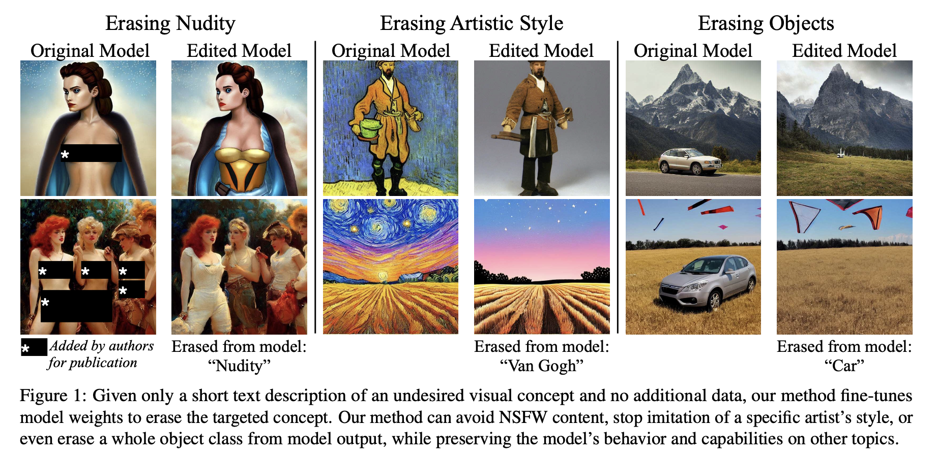
Goal: ESD aims to erase harmful concepts such as nudity, violence, or specific artist styles like “Van Gogh” from the generative models such as Stable Diffusion while maintaining the quality of the generated images for other concepts.
Approach: The authors proposed to alter the guiding signal regarding the concept to be erased to the one regarding the “null” concept (i.e., a neural prompt like “A photo”, “A person”), i.e., $\epsilon_\theta(z_t, c, t) \to \epsilon_\theta(z_t, c_{null}, t)$. The approach varies depending on whether the concept is directly expressible (such as “truck” or “dog”) or more abstract (like “nudity”). For direct concepts, modifications to the cross-attention layers of the diffusion model prove more effective, whereas abstract concepts necessitate adjustments to different layers for successful removal.

Central Optimization Problem

The central optimization problem is to reduce the probability of generating an image $x$ according to the likelihood that is described by the concept, scaled by a power factor $\eta$.

\[P_\theta(x) \propto \frac{P_{\theta^*}(x)}{P_{\theta^*}(c \mid x)^\eta}\]

where $P_{\theta^*}(x)$ is the distribution generated by the original model $\theta^*$ and $P_{\theta^*}(c \mid x)$ is the probability of the concept $c$ given the image $x$. The power factor $\eta$ controls the strength of the concept erasure. A larger $\eta$ means a stronger erasure. $\theta$ is the parameters of the model after unlearning the concept $c$.

It can be interpreted as: if the concept $c$ is present in the image $x$ in which $P_{\theta^*} (c \mid x)$ is high, then the likelihood of the image $x$ under the new model $P_{\theta} (x)$ will be reduced. While if the concept $c$ is not present in the image $x$ in which $P_{\theta^*} (c \mid x)$ is low, then the likelihood of the image $x$ under the new model $P_{\theta} (x)$ will be increased.

Because of the Bayes’ rule, the likelihood of the concept $c$ given the image $x$ can be rewritten as follows:

\[P_{\theta^*} (c \mid x) = \frac{P_{\theta^*} (x \mid c) P_{\theta^*} (c)}{P_{\theta^*} (x)}\]

Therefore, the above equation can be rewritten when taking the derivative w.r.t. $x$ as follows (you might need to rotate your phone to see the full equation ):

\[\nabla_{x} \log P_{\theta} (x) \propto \nabla_{x} \log P_{\theta^*} (x) - \eta \nabla_{x} \log P_{\theta^*} (c \mid x)\] \[\nabla_{x} \log P_{\theta} (x) \propto \nabla_{x} \log P_{\theta^*} (x) - \eta (\nabla_{x} \log P_{\theta^*} (x \mid c) + \nabla_{x} \log P_{\theta^*} (c) - \nabla_{x} \log P_{\theta^*} (x))\] \[\nabla_{x} \log P_{\theta} (x) \propto \nabla_{x} \log P_{\theta^*} (x) - \eta (\nabla_{x} \log P_{\theta^*} (x \mid c) - \nabla_{x} \log P_{\theta^*} (x))\]

Because in the diffusion model, each step has been approximated to a Gaussian distribution, therefore, the gradient of the log-likelihood is computed as follows:

\[\nabla_{x} \log P_{\theta^*} (x) = \frac{1}{\sigma^2} (x - \mu)\]

where $\mu$ is the mean of the diffusion model, $\sigma$ is the standard deviation of the diffusion model, and $c$ is the concept. Based on the repameterization trick, the gradient of the log-likelihood is correlated with the noise $\epsilon$ at each step as follows (linking between DDPM and the score-based matching ):

\[\epsilon_{\theta}(x_t,t) \propto \epsilon_{\theta^*} (x_t,t) - \eta (\epsilon_{\theta^*}(x_t,c,t) - \epsilon_{\theta^*} (x_t,t))\]

where $\epsilon_{\theta}(x_t,t)$ is the noise at step $t$ of the diffusion model after unlearning the concept $c$. Finally, to fine-tune the diffusion model from pretrained model $\theta^*$ to new cleaned model $\theta$, the authors proposed to minimize the following loss function:

\[\mathcal{L}(\theta) = \mathbb{E}_{x_0 \sim \mathcal{D}} \left[ \sum_{t=0}^{T-1} \left\| \epsilon_{\theta}(x_t,t) - \epsilon_{\theta^*} (x_t,t) + \eta (\epsilon_{\theta^*}(x_t,c,t) - \epsilon_{\theta^*} (x_t,t)) \right\|^2 \right]\]

where $x_0$ is the input image sampled from data distribution $\mathcal{D}$, $T$ is the number of steps of the diffusion model.

Instead of recursively sampling the noise $\epsilon_{\theta}(x_t,t)$ at every step, we can sample the time step $t \sim \mathcal{U}(0, T-1)$ and then sample the noise $\epsilon_{\theta}(x_t,t)$ at that time step. Therefore, the loss function can be rewritten as follows:

\[\mathcal{L}(\theta) = \mathbb{E}_{x_0 \sim \mathcal{D}} \left[ \left\| \epsilon_{\theta}(x_t,t) - \epsilon_{\theta^*} (x_t,t) + \eta (\epsilon_{\theta^*}(x_t,c,t) - \epsilon_{\theta^*} (x_t,t)) \right\|^2 \right]\]

where $t \sim \mathcal{U}(0, T-1)$.

Final Objective Function

However, in the paper, instead of using the above loss function, the author proposed to use the following loss function:

\[\mathcal{L}(\theta) = \mathbb{E}_{x_0 \sim \mathcal{D}} \left[ \left\| \epsilon_{\theta}(x_t,c,t) - \epsilon_{\theta^*} (x_t,t) + \eta (\epsilon_{\theta^*}(x_t,c,t) - \epsilon_{\theta^*} (x_t,t)) \right\|^2 \right]\]

where $t \sim \mathcal{U}(0, T-1)$.

The difference between the two loss functions is that the first loss function is computed based on the unconditional noise $\epsilon_{\theta}(x_t,t)$ at the time step $t$ while the second loss function is computed based on the noise $\epsilon_{\theta}(x_t,c,t)$ at the time step $t$ conditioned on the concept $c$.

Interpretation of the loss function: By minimizing the above loss function, we try to force the conditional noise $\epsilon_{\theta}(x_t,c,t)$ to be close to the unconditional noise $\epsilon_{\theta^*} (x_t,t)$ of the original model. Because the noise $\epsilon_{\theta^*} (x_t,t)$ is the signal to guide the diffusion model to generate the image $x_{t-1}$ (recall the denoising equation $x_{t-1} = \frac{1}{\sqrt{\alpha_t}}(x_t - \frac{1 - \alpha_t}{\sqrt{1 - \bar{\alpha}_t}} \epsilon_{\theta^*} (x_t,t)) + \sigma_t z$), therefore, by forcing the conditional noise $\epsilon_{\theta}(x_t,c,t)$ to be close to the unconditional noise $\epsilon_{\theta^*} (x_t,t)$, we try to force the diffusion model to generate the image $x_{t-1}$ close to the image generated without the concept $c$.

Note: In the above objective function, $x_t$ is the image from the training set $\mathcal{D}$ at time step $t$. However, as mentioned in the paper “We exploit the model’s knowledge of the concept to synthesize training samples, thereby eliminating the need for data collection”. Therefore, in the implementation, $x_t$ is the image generated by the fine-tuned model at time step $t$.

Editing Implicit Assumptions in Text-to-Image Diffusion Models (TIME)

Paper: https://arxiv.org/abs/2303.08084

Code: https://github.com/bahjat-kawar/time-diffusion

Summary TIME

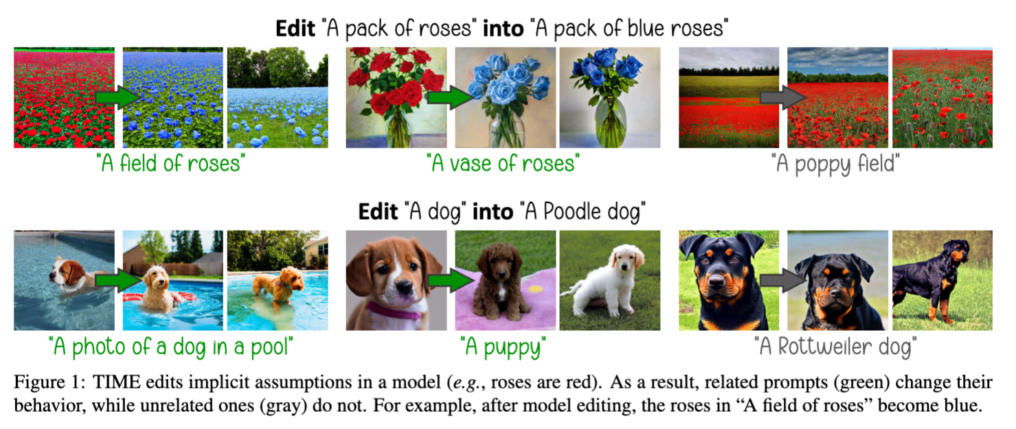
Goal: receives an under-specified “source” prompt (e.g., “A pack of roses”), which is requested to be well-aligned with a “destination” prompt (e.g., “A pack of blue roses”) containing an attribute that the user wants to promote (e.g., “blue roses”). After the editing, the model should change its behavior on only related prompts (e.g., image generated by a prompt “A field of roses” will be changed to red roses) while not affecting the characteristics or perceptual quality in the generation of different concepts (e.g., image generated by a prompt “A poppy field” will not be changed) (Ref to the figure above).
Implications: The change is expected to manifest in generated images for related concepts, while not affecting the characteristics or perceptual quality in the generation of different ones. This would allow us to fix incorrect, biased, or outdated assumptions that text-to-image models may make. For example, gender bias with the concept “doctor” or “teacher”. This method can also be used to erase harmful concepts such as “nudity” or “gun” from the model by mapping them to “safe/neutrual” concept like “flower” or “cat” or “null”.
Important this approach edits the projection matrices in the cross-attention layers to map the source prompt close to the destination, without substantially deviating from the original weights. Because these matrices operate on textual data irrespective of the diffusion process or the image contents, they constitute a compelling location for editing a model based on textual prompts.

Central Optimization Problem

Given a pretrain layer $W^{*}$, a set of concepts to be edited $E$ (i.e., “roses”, “doctor”, “nudity”), the goal is to find a new layer $W$ that is close to $W^{*}$ but does not contain any concept in $E$.

To do that, proposed to use the following optimization problem:

\[\underset{W}{\min} \sum_{c_i \in E} \| W c_i - v_i^* \|^2_2 + \lambda \| W - W^{*} \|^2_2\]

where $v_i^*$ is the targeted vector for concept $c_i$.

As derived in , the solution of this optimization problem is:

\[W = \left( \sum_{c_i \in E} v_i^* c_i^T + \lambda W^{*} \right) \left( \sum_{c_i \in E} c_i c_i^T + \lambda \mathbb{I} \right)^{-1}\]

By defining $v^*$ differently, the authors proposed 3 types of editing:

Erasing/Moderation: Choose $v^* = W c^*$, where $c^*$ is the targeted concept different from the concepts to be earased $c_i \in E$$. For example, harmful concept like “nudity” or “gun” can be erased to “safe/neutrual” concept like “flower” or “cat”, or artistic concept like “Kelly Mckernan” or “Van Gogh” to “non-artistic” concept like “art” or “ “.
Debiasing: Choose $v^* = W (c_i + \sum_{t=1}^p \alpha_t a_t)$ where $c_i$ is “doctor” and $a_t$ is attributes that we want to distribute across such as “white”, “asian”, “black”. By this way, the original concept “doctor” no longer only associated with “white” but also with “asian” and “black”.

Pros and Cons

Pros:

It does not require training or finetuning, it can be applied in parallel for all cross-attention layers, and it modifies only a small portion of the diffusion model weights while leaving the language model unchanged. When applied on the publicly available Stable Diffusion, TIME edits a mere 2.2% of the diffusion model parameters, does not modify the text encoder, and applies the edit in a fraction of a second using a single consumergrade GPU.

Cons:

It risks interference with surrounding concepts when editing a particular concept. For example, editing doctors to be female might also affect teachers to be female. .
TIME has a regularization term that prevents the edited matrix from changing too radically. However, it is a general term and thus affects all vector rep- resentations equally. The follow-up work of proposes an alternative preservation term that allows targeted editing of the parameters of the pretrained generative model while maintaining its core capabilities.

Unified Concept Editing in Diffusion Models

Accepted to WACV 2024. https://arxiv.org/pdf/2308.14761.pdf
Affiliation: Northeastern University, Technion and MIT. Same group with the ESD paper.
Link to Github: https://github.com/rohitgandikota/unified-concept-editing

Summary UCE

It is a follow-up work of that proposes an alternative preservation term that allows targeted editing of the parameters of the pretrained generative model while maintaining its core capabilities.

Central Optimization Problem

Given a pretrain layer $W^{*}$, a set of concepts to be edited $E$ and a set of concepts to be preserved $P$, the goal is to find a new layer $W$ that is close to $W^{*}$ but does not contain any concept in $E$ and preserve all concepts in $P$.

To do that, proposed to use the following optimization problem:

\[\underset{W}{\min} \sum_{c_i \in E} \| W c_i - v_i^* \|^2_2 + \sum_{c_j \in P} \| W c_j - W^* c_j \|^2_2\]

where $v_i^*$ is the targeted vector for concept $c_i$.

As derived in , the solution of this optimization problem is:

\[W = \left( \sum_{c_i \in E} v_i^* c_i^T + \sum_{c_j \in P} W^* c_j cj^T \right) \left( \sum_{c_i \in E} c_i c_i^T + \sum_{c_j \in P} c_j c_j^T \right)^{-1}\]

By defining $v^*$ differently, the authors proposed 3 types of editing:

Erasing/Moderation: Choose $v^* = W c^*$, where $c^*$ is the targeted concept different from the concepts to be earased $c_i \in E$$. For example, harmful concept like “nudity” or “gun” can be erased to “safe/neutrual” concept like “flower” or “cat”, or artistic concept like “Kelly Mckernan” or “Van Gogh” to “non-artistic” concept like “art” or “ “.
Debiasing: Choose $v^* = W (c_i + \sum_{t=1}^p \alpha_t a_t)$ where $c_i$ is “doctor” and $a_t$ is attributes that we want to distribute across such as “white”, “asian”, “black”. By this way, the original concept “doctor” no longer only associated with “white” but also with “asian” and “black”.

Pros and Cons

Pros:

Fast and efficient. It can finish the editing in less than 5 minutes on a single V100 GPU (Compared to 1 hour for the ESD method). The editing performance in some settings (e.g., erasing object-related concepts such as “trucks”, “tench”) is better than the ESD method.

Poor performance The performance on erasing concepts is still limited. As I reproduced the experiment to erase artist concept call “Kelly Mckernan” and compare with the original model, the two generated images from two models are still very similar.

Limited Expressiveness The authors use textual prompt as the input to specify the concept to be erased, e.g., “Kelly Mckernan” or “Barack Obama” or “nudity”. However, a concept can be described in many different ways, for example, “Barack Obama” can be described as “the 44th president of the United States” or “the first African American president of the United States”. Therefore, it is not possible to erase all concepts related to “Barack Obama” by just erasing the keyword “Barack Obama”.

Unaware of the time step In this formulation, the authors just proposed to rewrite the projection matrices $W_K$ and $W_V$ of the attention layer $W$ independently and ignore the query matrix $W_Q$. However, the query ouput $W_Q x$ has the information about the time step $t$ of the diffusion model.

Unknown preserved concepts In term of methodology, while there is a closed-form solution for the optimization problem, it is not clear how to solve the optimization problem when the number of preserved concepts is large and even uncountable (i.e., how we can know how many concept that Stable Diffusion can generate?). In fact, I have tried to run the experiment to erase 5 concepts from the ImageNette dataset while not specifying the preserved concepts. While the erasing rate can be 100\%, the preserving rate is low, especially for those concepts that are not specified to be preserved.

Invertibility issue If we just ignore the preserved concepts, the optimization problem is still problematic.

\[W = \left( \sum_{c_i \in E} v_i^* c_i^T \right) \left( \sum_{c_i \in E} c_i c_i^T \right)^{-1}\]

where $v_i^*$ is the targeted vector for concept $c_i$.

Let’s dig deeper into this OP. As mentioned in the paper, $v_i^*=W^* c_{tar}$ where $c_{tar}$ is the targeted concept different from the concepts to be earased $c_i \in E$$ such as “nudity” or “gun” can be erased to “safe/neutrual” concept like “flower” or “cat”, or artistic concept like “Kelly Mckernan” or “Van Gogh” to “non-artistic” concept like “art” or “ “.

In implementation, $c_i$ and $c_{tar}$ are input of the attention layer $W$ which are ouput of the text encoder, therefore, they are unchanged during the optimization process.

Therefore, the optimization problem can be rewritten as follows:

\[W = \left( \sum_{c_i \in E} W^* c_{tar} c_i^T \right) \left( \sum_{c_i \in E} c_i c_i^T \right)^{-1}\]

where $W^* c_i$ is the projected vector.

As mentioned in Appendix A of the paper, one condition to ensure that the optimization problem has a solution is that the matrix $\sum_{c_i \in E} c_i c_i^T$ is invertible. To ensure this condition, the authors proposed to add $d$ additional preservation terms along the canonical basis vectors (i.e., adding identity matrix) as follows:

\[W = \left( \sum_{c_i \in E} W^* c_{tar} c_i^T \right) \left( \sum_{c_i \in E} c_i c_i^T + \lambda I \right)^{-1}\]

where $\lambda$ is a regularization factor and $I$ is the identity matrix. While this trick can ensure the invertibility, it can be seen that these additional preservation terms can affect the projection of the concepts to be erased $c_i \in E$ and thus affect the erasing process (i.e., too big $\lambda$)

Recall some basic linear algebra:

$c_i$ is a vector with $d$ dimensions, therefore, $c_i c_i^T$ is a matrix with $d \times d$ dimensions.

W is a projection matrix with $d_o \times d$ dimensions, therefore, $W c_i$ is a vector with $d_o$ dimensions and $W c_i c_i^T$ is a matrix with $d_o \times d$ dimensions.

If $c_i$ is a non-zero vector, then $c_i c_i^T$ has rank 1. Therefore, $\sum_{c_i \in E} c_i c_i^T$ has rank at most $\min(\mid E \mid, d)$.

what is the canonical basic vectors?

The canonical basis vectors are the vectors with all components equal to zero except for one component equal to one. For example, in $\mathbb{R}^3$, the canonical basis vectors are $e_1 = (1, 0, 0)$, $e_2 = (0, 1, 0)$ and $e_3 = (0, 0, 1)$.

Circumventing Concept Erasure Methods For Text-to-Image Generative Models

Paper: https://openreview.net/forum?id=ag3o2T51Ht
Accepted to ICLR 2024

Summary

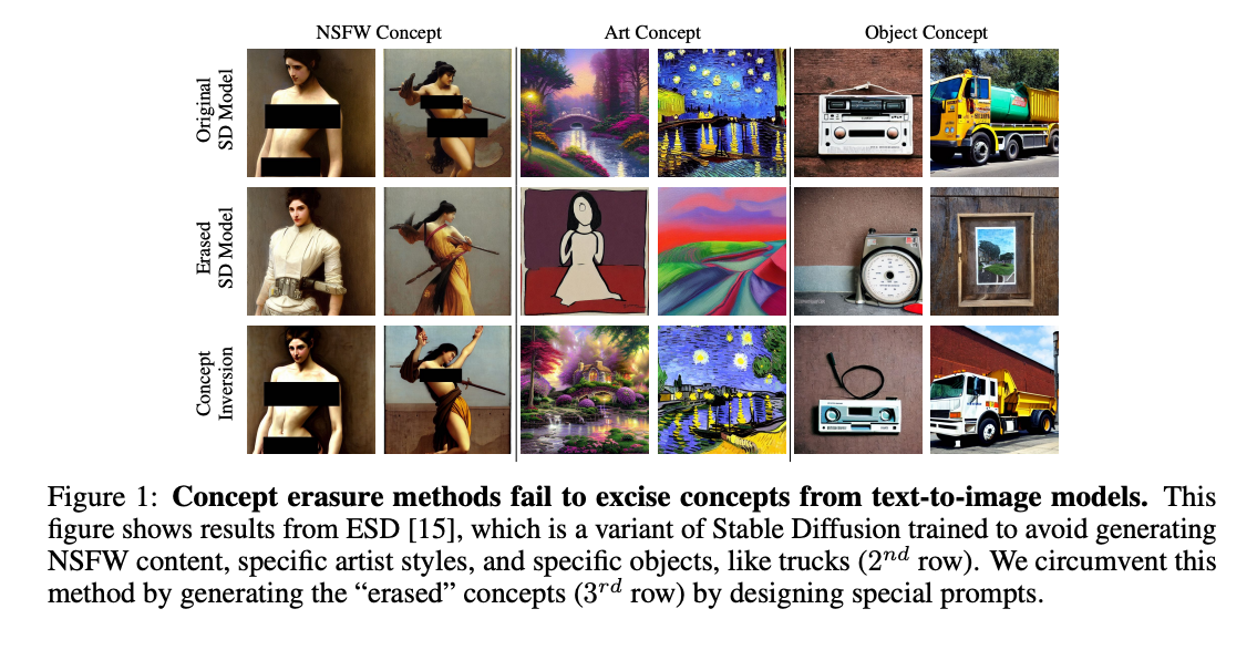
The paper proposes a method called Concept Inversion to circumvent 7 recent concept erasure methods for text-to-image generative models including Erased Stable Diffusion , Selective Amnesia , Forget-me-not , Ablating Concepts , Unified Concept Editing , Negative Prompt , and Safe Latent Diffusion . The authors show that with even with zero training or fine-tuning the pretrained erased model, it is possible to generate the erased concept with a suitably constructed prompt.
The authors utilized the Textual Inversion technique to find special word embeddings that can recover the erased concepts. The method is simply yet effective showing that existing concept erasure methods actually perform some form of concept hiding or textually obfuscating rather than concept erasure. For example, while the erased model may not generate images of “nudity” when prompted with a word “nudity”, it can still generate images of “nudity” when prompted with a special phrase “a person without clothes”. We can intuitively understand the approach is find a special embedding $S^{*}$ that represents these special phrases by inversing some images with the erased concept and then use this special embedding to generate the erased concept like “A person $S^{*}$”.
Cons Because using the Textual Inversion technique, this method needs to replace the original Embedding Lookup table so that it can map the placeholder $S^{*}$ to the special embedding $v^{*}$.

Recall the Textual Inversion technique :

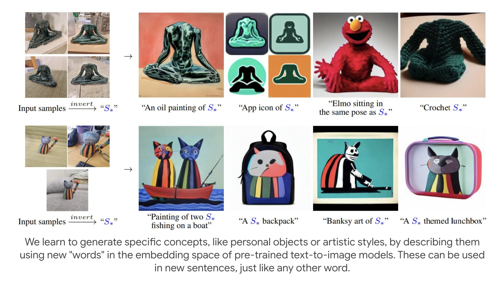
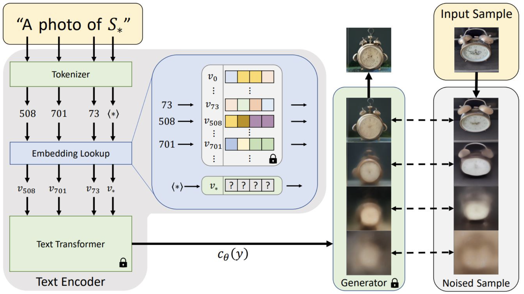
Given a pretrained text-to-image generative model (Unet) $\epsilon_\theta$, textual encoder $c_\phi$ (denoted as $c_\theta$ as the figure above, but it seems to be confused with the Unet $\epsilon_\theta$) and set of target images $X$, and a specific text placeholder $S^{*}$ that corresponds to a specific textual embedding vector $v^{*}$, the goal is to find the special textual embedding vector $v^{*}$ that can reconstruct the input image $x \sim X$. The authors proposed to use the following optimization problem which is the same as the DDPM model but with the special placeholder/prompt $S^{*}$:

\[v^{*} = \underset{v}{\arg\min} \; \mathbb{E}_{z \sim \varepsilon(x), x \sim X, \epsilon \sim \mathcal{N}(0,I), t} [ \|\epsilon - \epsilon_\theta (z_t, c_\phi(v), t) \|_2^2 ]\]

where $v$ is the textual embedding vector $v = \text{Lookup}(S^{*})$.

Adapt to the concept erasure problem

Given the background of the Textual Inversion technique, it is just straightforward to adapt this technique to circumvent the concept erasure problem. Most of the concept erasure methods are hacked by standard Textual Inversion. More details can be found in the paper. One important thing is that the authors need to have a set of target images $X$ that contains the erased concept. The authors made an assume that the adversary can access a small number of examples of the targeted concept from Google Images, specifically, 6 samples for art style concept (e.g., Van Gogh), 30 samples for object concept (e.g., cassette player), and 25 samples for ID concept (e.g., Angelina Jolie).