Visual Prompt Tuning
Resources:
About the paper
Key ideas:
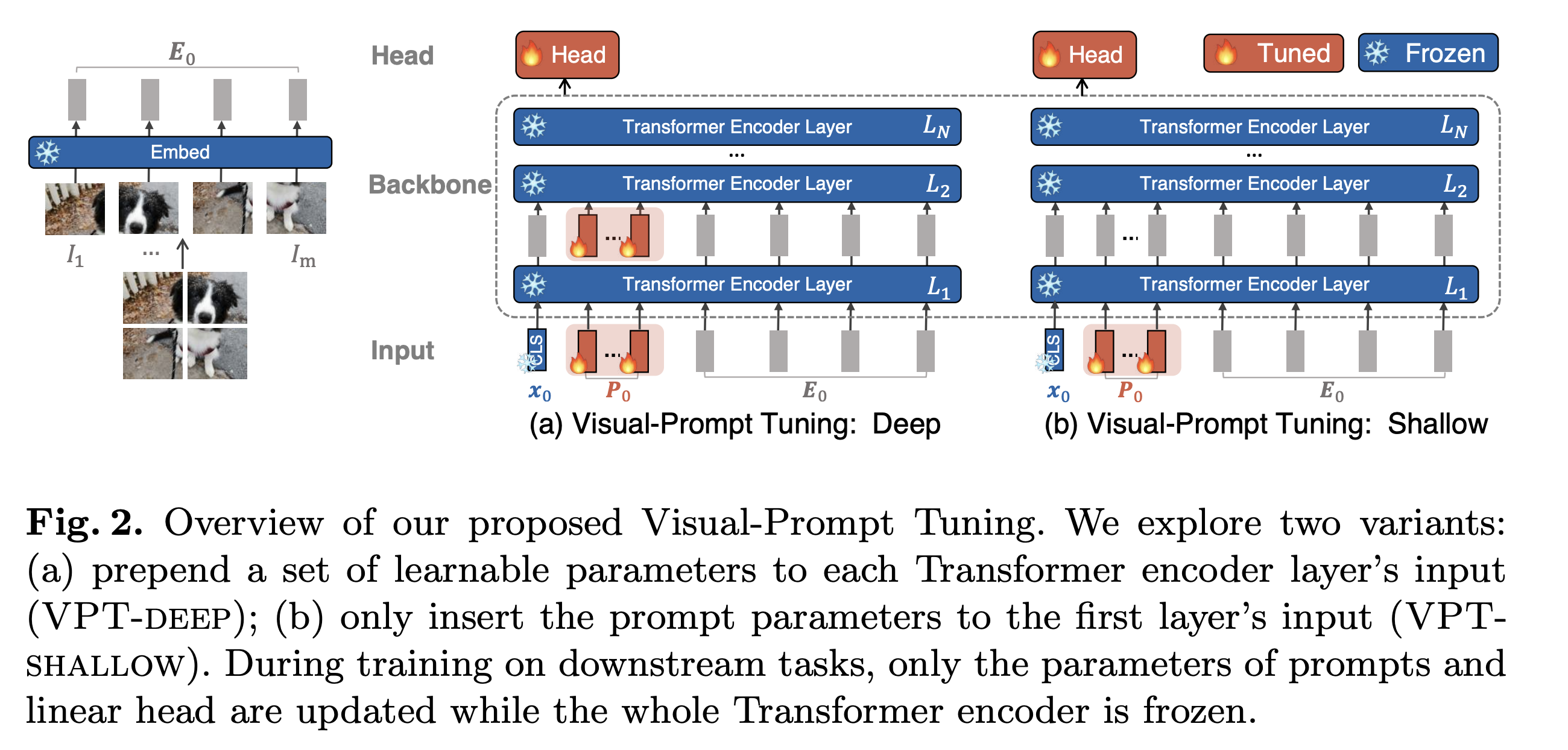
- Introducing an additional trainable input (similar as adversarial examples) in additional to the original input. The new input will be treated as the same as the original input without the need of changing model architecture.
- During fine-tuning phase, only fine-tune/update the prompt while frozing the backbone model in order to minimize the objective loss.
Background
Foundation models is a very big model, which was trained of massive unlabeled data, usually by using self-supervised learning methods.
In computer vision problems, most SOTA results now are achieved by adapting large foundation models (i.e., CLIP or Stable Diffusion or Segment Anything Model) to the downstream tasks. Full fine-tuning invovles updating all the backbone parameters, which is often the most effective adapting method. However, it has several drawbacks: (1) store and deploy a separate copy of the backbone parameters for every single task, (2) do not have enough data. LORA
Prompt tuning is a common technique in NLP, in which additional prompts (e.g., several trainable word embeddings) are added in addition to original input sequence. The advantage of prompt tuning is that we can use the same backbone model with the new sequences, thanks to the attention machenism.
Method

ViT and Multiheaded Self-Attention (MSA)
For a plain Vision Transformer (ViT) with \(N\) layers, for each layer \(L_i\), the output is simply formulated as follows:
\[[x_i, E_i] = L_i \left( \left[ x_{i-1}, E_{i-1} \right] \right)\]where \(x_i \in \mathbb{R}^d\) denotes \([CLS]\)’s embedding at \(L_{i+1}\)’s input space. \(E_i = \{ e_i^j \}_{j=1}^m\) which is a collection of \(m\) image patch embeddings from layer \(E_i\). All togerther, at each layer, its taks \(m+1\) embeddings \(\left[ x_{i-1}, E_{i-1} \right]\) and returns the same amount \([x_i, E_i] \in \mathbb{R}^{ (1+m) \times d}\).
The classification head is used to map the final layer’s \([CLS]\) embedding, \(x_N\) , into a predicted class probability distribution \(y = \text{Head} (x_N)\).
Visual-Prompt Tuning
The authors introduced two variants: VPT-Shallow whereas the prompt is added into the first layer only and VPT-Deep whereas \(N\) trainable, distinct prompts are added into each corresponding layers.
VPT-Shallow
\([x_1, Z_1, E_1] = L_1 (x_0, P, E_0)\)
\([x_i, Z_i, E_i] = L_1 (x_{i-1}, Z_{i-1}, E_{i-1}) \; \forall \; i = 2, 3, ..., N\)
\(y = \text{Head} (x_N)\)
VPT-Deep
\([x_i, Z_i, E_i] = L_1 (x_{i-1}, Z_{i-1}, E_{i-1}) \; \forall \; i = 1, 2, 3, ..., N\)
\(y = \text{Head} (x_N)\)
Results
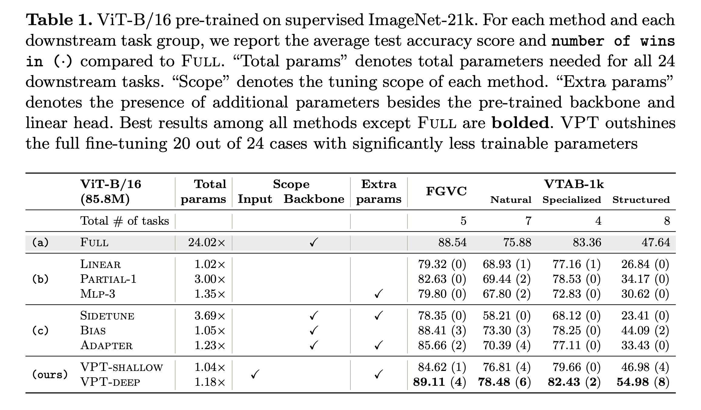
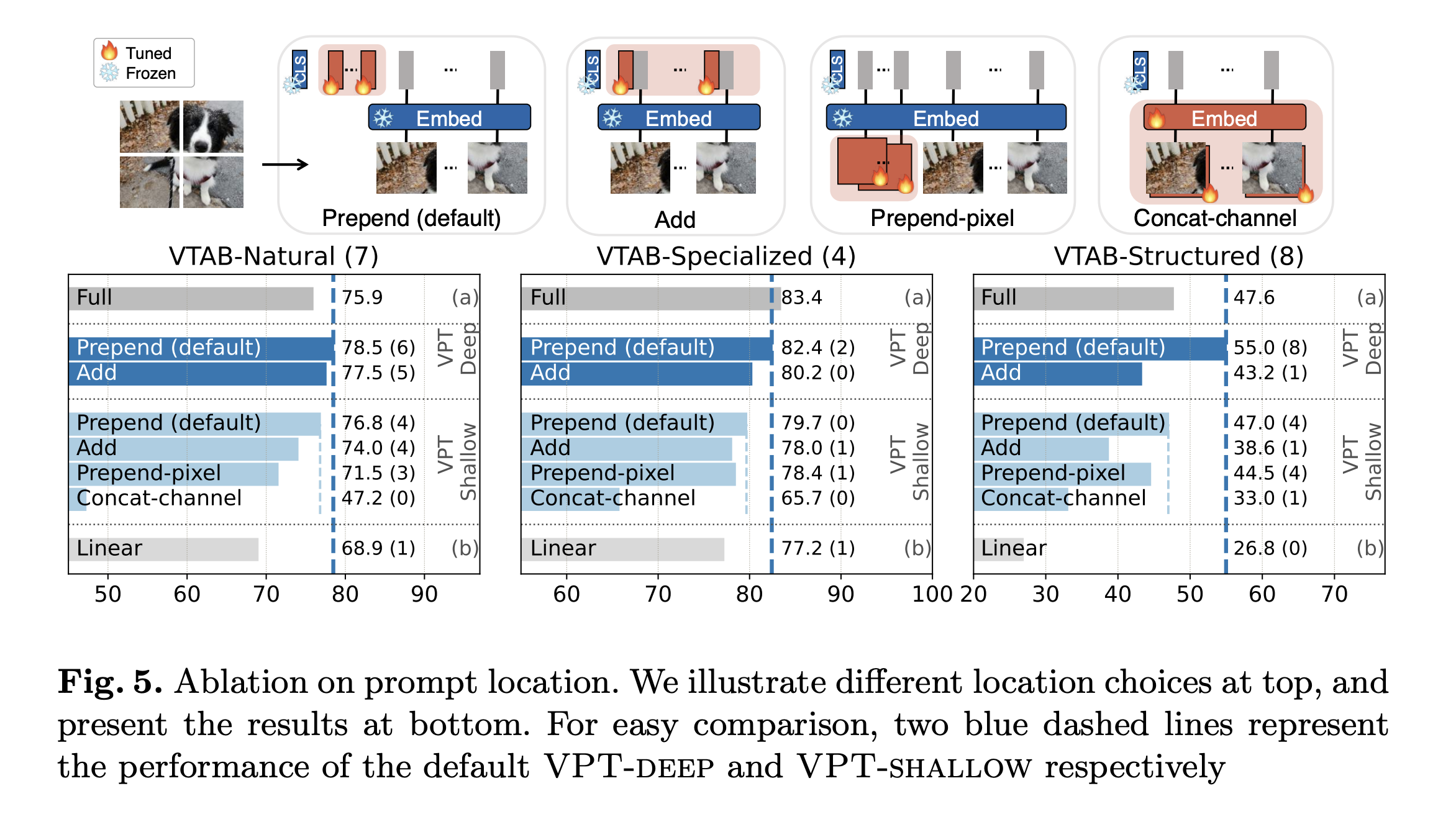
Some key results as below:
VPT-Deep significantly outperforms VPT-Shallow

Prepend or Add Adding performance generally falls behind with the default Prepend in both deep and shallow settings.

Prompt depth the results suggest that prompts at earlier Transformer layers matter more than those at later layers. Adding prompts to majority of layers (9/12 or 12/12 layers) is better than adding prompts to fewer layers.
Enjoy Reading This Article?
Here are some more articles you might like to read next: