Coding Series - Part 1 - Data Structure and Algorithms Foundation
Sorting Algorithms
References:
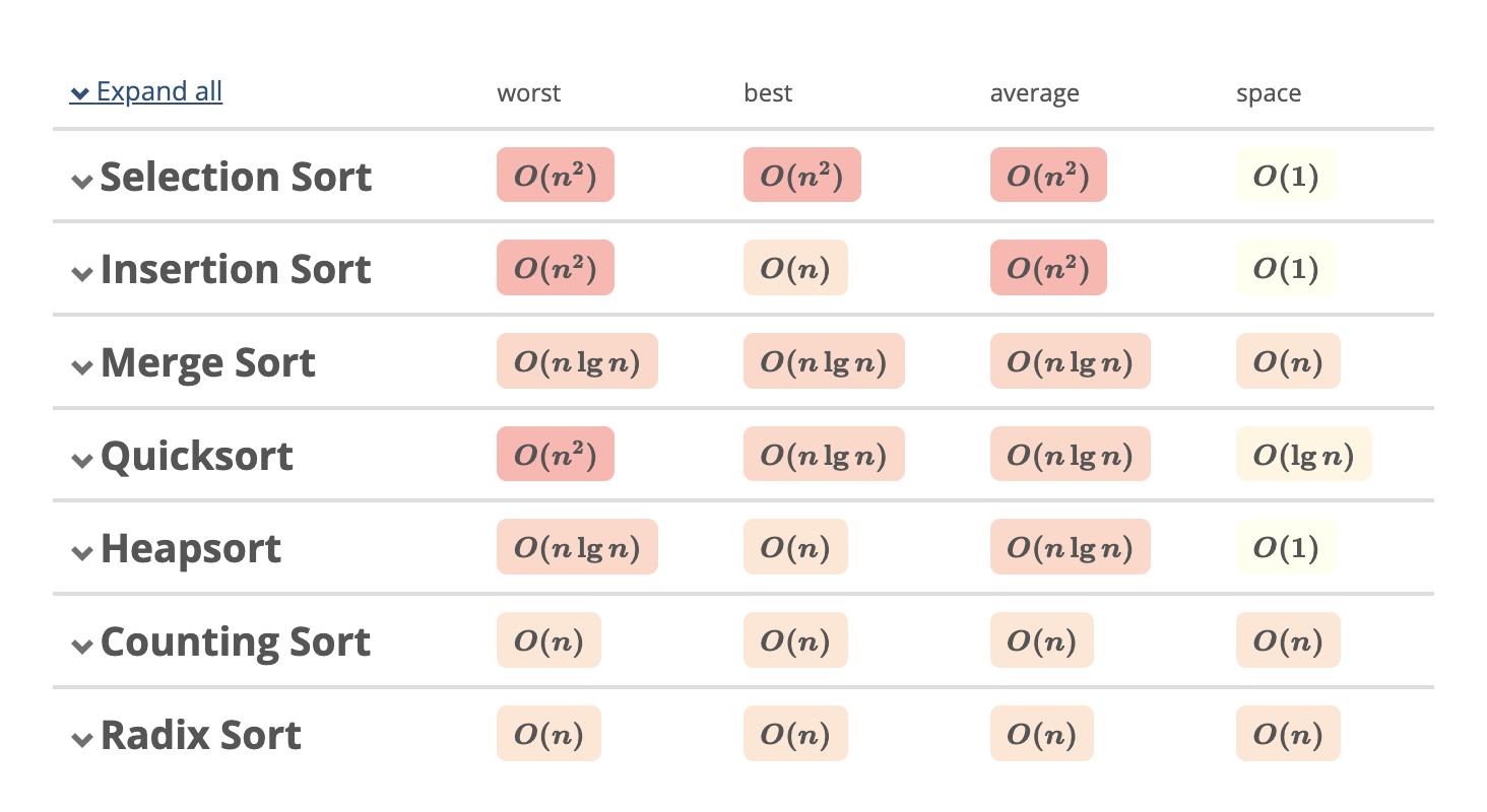
Sorting is the process of arranging data in a specific order. The most common orders are numerical order (ascending or descending) and lexicographical order (dictionary order).
Beside the time complexity and space complexity, we also need to consider the stability - whether the relative order of equal elements is preserved. For example, in sorting students by grade, keeping names in alphabetical order, stable sorting algorithms like Merge Sort, Insertion Sort and Bubble Sort are preferred.
Common Sorting Algorithms
Selection Sort
Selection sort works by repeatedly “selecting” the next-smallest element from the unsorted array and moving it to the front.

Time Complexity: The time complexity of selection sort is \(O(n^2)\) in all cases, even when the array is already sorted.
def selection_sort(arr):
    for i in range(len(arr)):
        min_idx = i
        for j in range(i+1, len(arr)):
            if arr[j] < arr[min_idx]:
                min_idx = j
        arr[i], arr[min_idx] = arr[min_idx], arr[i]
    return arr
Bubble Sort
Bubble sort works by repeatedly swapping the adjacent elements if they are in the wrong order.
Time Complexity: The time complexity of bubble sort is \(O(n^2)\) in the worst case and \(O(n)\) in the best case when the array is already sorted.
def bubble_sort(arr):
    n = len(arr)
    for i in range(n):
        for j in range(0, n-i-1):
            if arr[j] > arr[j+1]:
                arr[j], arr[j+1] = arr[j+1], arr[j]
    return arr
Insertion Sort
Insertion sort works by inserting elements from an unsorted array into a sorted subsection of the array.

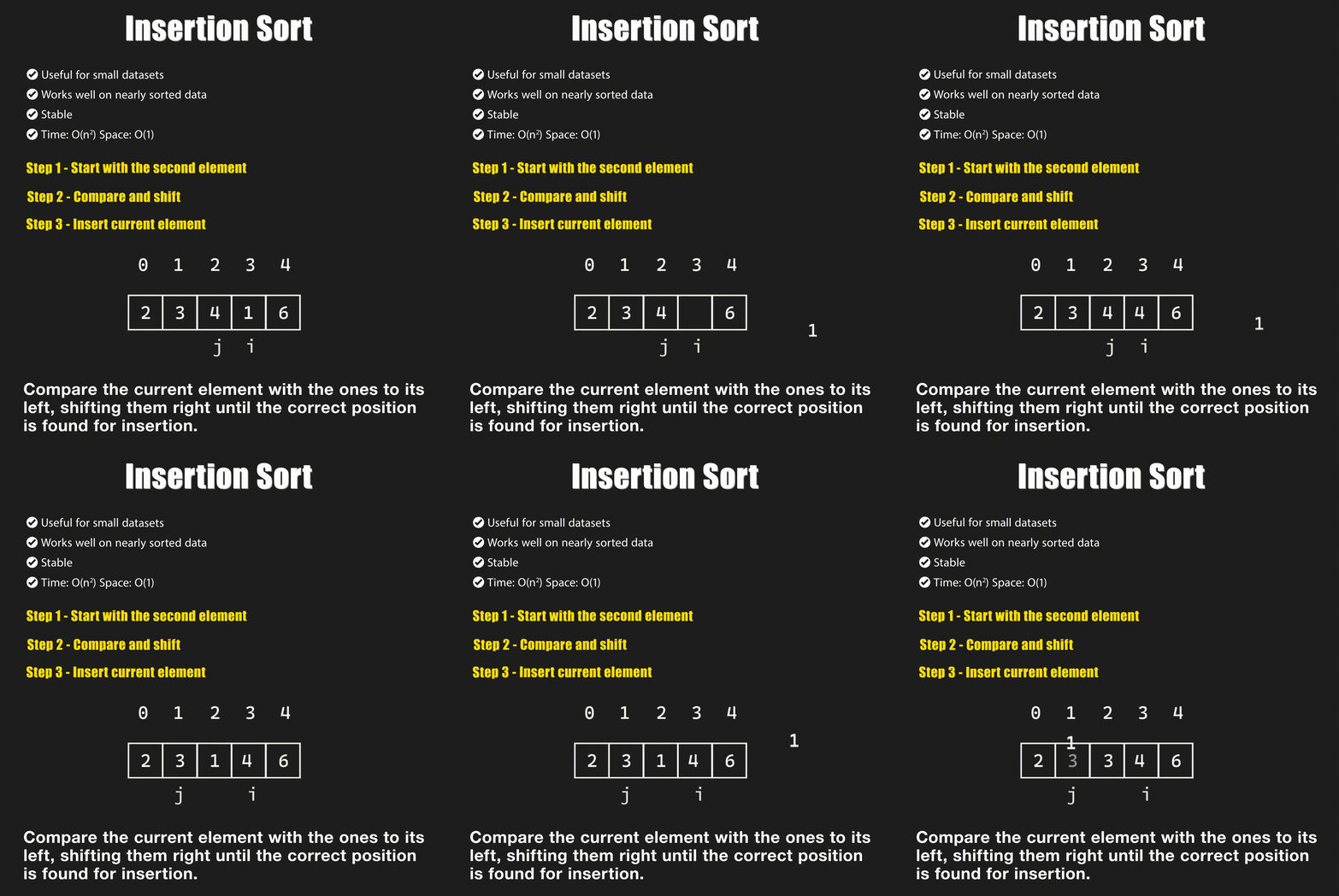
Time Complexity: The time complexity of insertion sort is \(O(n^2)\) in the worst case (sorted in reverse order), but \(O(n)\) in the best case when the array is already sorted.
def insertion_sort(arr):
    for i in range(1, len(arr)):
        key = arr[i]
        j = i - 1
        while j >= 0 and key < arr[j]:
            arr[j + 1] = arr[j]
            j -= 1
Merge Sort
Merge sort works by dividing the array into two halves, sorting each half, and then merging the two halves.

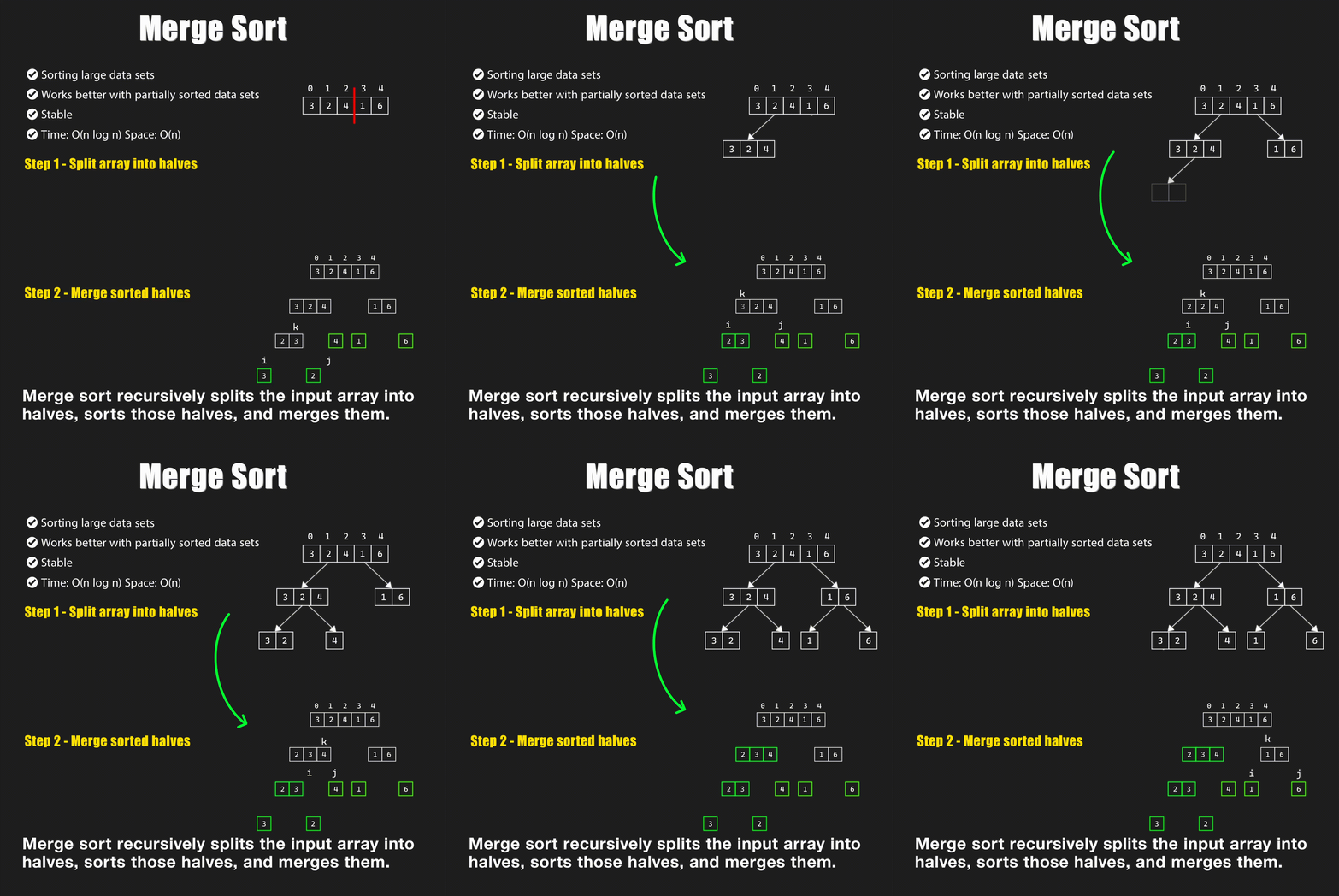
Time Complexity: The time complexity of merge sort is \(O(n \log n)\) in all cases. The \(\log n\) comes from the divide step, and the \(n\) comes from the conquer step. The space complexity is \(O(n)\) due to the additional array used for merging.
def merge_sort(arr):
    if len(arr) <= 1:
        return arr
    mid = len(arr) // 2
    left = merge_sort(arr[:mid])
    right = merge_sort(arr[mid:])
    return merge(left, right)

def merge(left, right):
    result = []
    i = j = 0
    while i < len(left) and j < len(right):
        if left[i] < right[j]:
            result.append(left[i])
            i += 1
        else:
            result.append(right[j])
            j += 1
    result.extend(left[i:])
    result.extend(right[j:])
    return result
Quick Sort
Quick sort works by selecting a “pivot” element from the array and partitioning the other elements into two sub-arrays, according to whether they are less than or greater than the pivot.
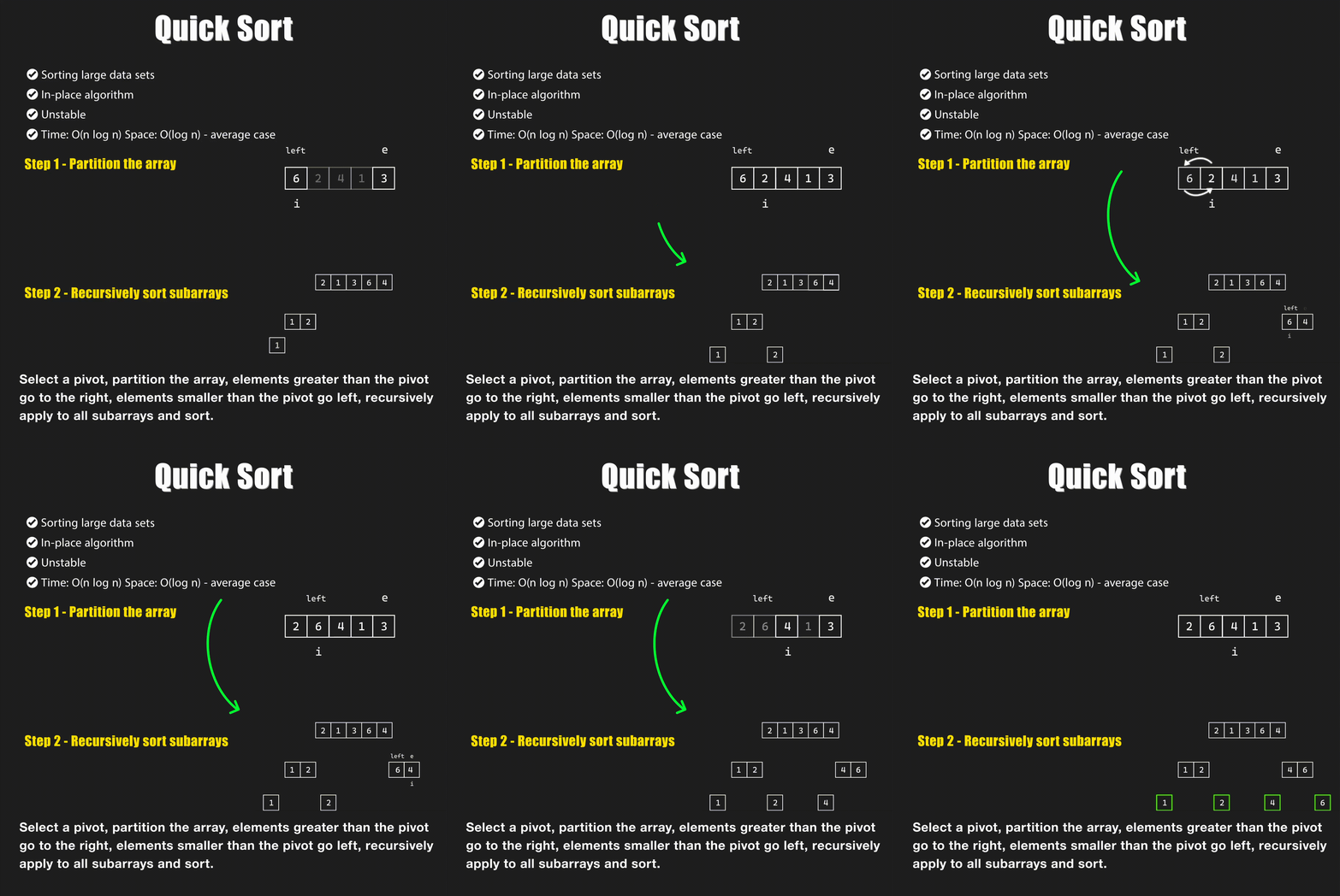
Time Complexity: The time complexity of quick sort is \(O(n \log n)\) in the best case, \(O(n^2)\) in the worst case, and \(O(n \log n)\) in the average case. The space complexity is \(O(\log n)\) due to the recursive call stack.
def quick_sort(arr):
    if len(arr) <= 1:
        return arr
    pivot = arr[len(arr) // 2]
    left = [x for x in arr if x < pivot]
    middle = [x for x in arr if x == pivot]
    right = [x for x in arr if x > pivot]
    return quick_sort(left) + middle + quick_sort(right)
Heap Sort
Heap sort works by building a heap from the array and then repeatedly extracting the maximum element from the heap.
import heapq

def heap_sort(arr):
    heapq.heapify(arr)
    return [heapq.heappop(arr) for _ in range(len(arr))]
Time Complexity: The time complexity of heap sort is \(O(n \log n)\) in all cases. The space complexity is \(O(1)\) due to the in-place sorting.
Lambda Function
Lambda function is a small anonymous function using the lambda keyword. It can have any number of arguments, but can only have one expression.
When combined with the sorted() function, we can sort the data based on a specific condition.
lambda arguments: expression
Example: Given a list of strings, sort them by the length of the strings first, and then by the alphabetical order.
strings = ["apple", "banana", "cherry", "date"]
sorted_strings = sorted(strings, key=lambda x: (len(x), x))
print(sorted_strings)
Searching Algorithms
Searching is the process of finding a specific element in a data structure. The data structure can be an array, a linked list, a tree, or a graph. There are two main types of searching algorithms: linear search and binary search, along with special cases like Breadth-First Search (BFS) and Depth-First Search (DFS).
Linear Search
Linear search works by iterating through the data structure and comparing each element to the target value.
Time Complexity: The time complexity of linear search is \(O(n)\) in the worst case.
def linear_search(arr, target):
    for i, element in enumerate(arr):
        if element == target:
            return i
    return -1
Binary Search
Binary search works by repeatedly dividing the search interval in half. If the value of the search key is less than the item in the middle of the interval, narrow the interval to the lower half. Otherwise, narrow it to the upper half.
Time Complexity: The time complexity of binary search is \(O(\log n)\) in the worst case, \(O(1)\) in the best case when the target is found, and \(O(\log n)\) in the average case.
def binary_search(arr, target):
    left, right = 0, len(arr) - 1
    while left <= right:
        mid = (left + right) // 2
        if arr[mid] == target:
            return mid
        elif arr[mid] < target:
            left = mid + 1
        else:
            right = mid - 1
    return -1
Breadth-First Search (BFS)
BFS works by exploring all the neighbors of a node before moving on to the next level of nodes. There are two things to consider:
- How to traverse the tree?
- How to keep track of the nodes that have been visited or not to avoid infinite loops?
In the code snippet below, we use a queue to store the nodes to be visited. When we visit a node, we enqueue its left and right children to the queue. We then dequeue the node from the queue and print its value. We repeat this process until the queue is empty.
Time Complexity: The time complexity of BFS in a binary tree is \(O(n)\) in the worst case, where \(n\) is the number of nodes in the tree.
from collections import deque

def bfs(root):
    queue = deque([root])
    while queue:
        node = queue.popleft()
        print(node.val) # Doing something with the node
        if node.left:
            queue.append(node.left)
        if node.right:
            queue.append(node.right)
Depth-First Search (DFS)
DFS works by exploring as far as possible along each branch before backtracking. Unlike BFS, we don’t need to keep track of the nodes that have been visited or not. We use recursion to traverse the tree.
Time Complexity: The time complexity of DFS in a binary tree is \(O(n)\) in the worst case, where \(n\) is the number of nodes in the tree.
def dfs(node):
    if node is None:
        return
    print(node.val) # Doing something with the node
    dfs(node.left)
    dfs(node.right)
Preorder Traversal: The root node is visited first, then the left subtree, and then the right subtree.
def preorder_traversal(node):
    if node is None:
        return
    print(node.val) # Doing something with the node
    preorder_traversal(node.left)
    preorder_traversal(node.right)
Inorder Traversal: The left subtree is visited first, then the root node, and then the right subtree.
def inorder_traversal(node):
    if node is None:
        return
    inorder_traversal(node.left)
    print(node.val) # Doing something with the node
    inorder_traversal(node.right)
Postorder Traversal: The left subtree is visited first, then the right subtree, and then the root node.
def postorder_traversal(node):
    if node is None:
        return
    postorder_traversal(node.left)
    postorder_traversal(node.right)
    print(node.val) # Doing something with the node
Two-Pointer Technique
The two-pointer technique is a common algorithm pattern used to solve problems involving arrays or linked lists. It involves using two pointers to traverse the data structure and find a solution. It is often used to check if a linked list has a cycle or to find the middle element of a linked list.
Example 1: Two-sum problem - searching for a pair of numbers in an array that add up to a given target.
def two_sum(arr, target):
    left, right = 0, len(arr) - 1
    while left < right:
        if arr[left] + arr[right] == target:
            return [left, right]
        elif arr[left] + arr[right] < target:
            left += 1
        else:
            right -= 1
Example 2: Checking if a linked list has a cycle.
def has_cycle(head):
    slow, fast = head, head
    while fast and fast.next:
        slow = slow.next
        fast = fast.next.next
        if slow == fast:
            return True
    return False
Example 3: Finding the middle element of a linked list.
def find_middle(head):
    slow, fast = head, head
    while fast and fast.next:
        slow = slow.next
        fast = fast.next.next
    return slow
Dynamic Programming
Dynamic programming is a method for solving a complex problem by breaking it down into simpler subproblems.
Fibonacci Sequence
The Fibonacci sequence is a series of numbers where each number is the sum of the two preceding ones, starting from 0 and 1.
def fibonacci(n):
    if n <= 1:
        return n
    return fibonacci(n-1) + fibonacci(n-2)
Longest Common Subsequence (LCS)
The longest common subsequence (LCS) problem is to find the longest subsequence that is present in two given sequences in the same order.
def lcs(str1, str2):
    m = len(str1)
    n = len(str2)
    dp = [[0] * (n+1) for _ in range(m+1)]
    for i in range(1, m+1):
        for j in range(1, n+1):
            if str1[i-1] == str2[j-1]:
                dp[i][j] = dp[i-1][j-1] + 1
            else:
                dp[i][j] = max(dp[i-1][j], dp[i][j-1])
    return dp[m][n]
Subsequence Pattern Matching
Given two strings str1 and str2, check if str1 is a subsequence of str2. The subsequence can be non-continuous, for example, “ace” is a subsequence of “abcde” but “aec” is not.
def is_subsequence(str1, str2):
    if len(str1) == 0:
        return True
    if len(str2) == 0:
        return False
    if str1[0] == str2[0]:
        return is_subsequence(str1[1:], str2[1:])
    else:
        return is_subsequence(str1, str2[1:])
Data Structures
Array
🔹 Definition: A collection of elements stored at contiguous memory locations.
🔹 Operations: Accessing (O(1)), Searching (O(n) or O(log n)), Insertion/Deletion (O(n))
arr = [1, 2, 3, 4, 5]
arr[0] # O(1)
arr.index(3) # O(n)
arr.append(6) # O(1)
arr.insert(0, 0) # O(n)
arr.remove(3) # O(n)
📌 Common Questions
- Two Sum → Find two numbers in an array that add up to a target sum. (Two-Pointer or HashMap)
- Best Time to Buy and Sell Stock → Find the maximum profit from stock prices. (Kadane’s Algorithm)
- Subarray Sum Equals K → Find a contiguous subarray whose sum equals K. (Prefix Sum + HashMap)
- Find Duplicate in an Array → Find the duplicate element in an array of N+1 numbers. (Floyd’s Cycle Detection)
- Merge Intervals → Given overlapping intervals, merge them. (Sorting + Greedy Approach)
Linked List
🔹 Definition: A linear data structure where elements (nodes) are linked using pointers.
🔹 Types: Singly, Doubly, Circular
🔹 Operations: Traversal (O(n)), Insertion/Deletion (O(1) at head), Searching (O(n))
class Node:
    def __init__(self, value):
        self.value = value
        self.next = None

# Creating a linked list
head = Node(1)
head.next = Node(2)
head.next.next = Node(3)

# Inserting a node at the head
new_head = Node(0)
new_head.next = head
head = new_head

# Deleting a node
head.next = head.next.next

# Searching for a node
current = head
target = 3
while current:
    if current.value == target:
        print("Found")
        break
    current = current.next
Tree
🔹 Definition: A non-linear data structure with nodes having at most two children (left and right).
🔹 Types: Binary Search Tree (BST), AVL Tree, Heap, Trie
🔹 Operations: Traversal (O(n)), Insertion/Deletion (O(log n)), Searching (O(log n))
class TreeNode:
    def __init__(self, value):
        self.value = value
        self.left = None
        self.right = None

# Creating a binary search tree
root = TreeNode(5)
root.left = TreeNode(3)
root.right = TreeNode(7)

# Inserting a node
root.left.left = TreeNode(1)

# Deleting a node
root.right = None

# Searching for a node
def dfs(node, target):
    if node is None:
        return None
    if node.value == target:
        return node
    return dfs(node.left, target) or dfs(node.right, target)

dfs(root, 3)
Trie
Source: https://www.geeksforgeeks.org/trie-insert-and-search/
What is Trie?In short, Trie is a k-ary tree where k is the largest number of children of a node.
Because of its structure, Trie is an efficient information retrieval data structure. Using Trie, search complexities can be brought to optimal limit (key length). If we store keys in binary search tree, a well balanced BST will need time proportional to M * log N, where M is maximum string length and N is number of keys in tree. Using Trie, we can search the key in O(M) time. However the penalty is on Trie storage requirements.
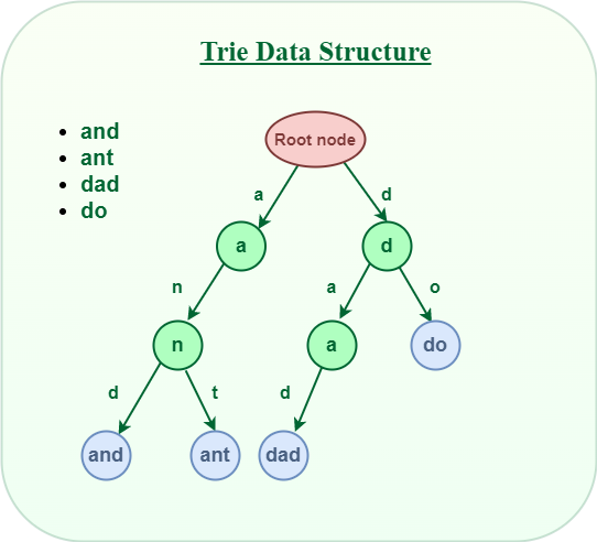
The following code is a simple Trie for English alphabet.
class TrieNode:

    # Trie node class
    def __init__(self):
        self.children = [None]*26

        # isEndOfWord is True if node represent the end of the word
        self.isEndOfWord = False
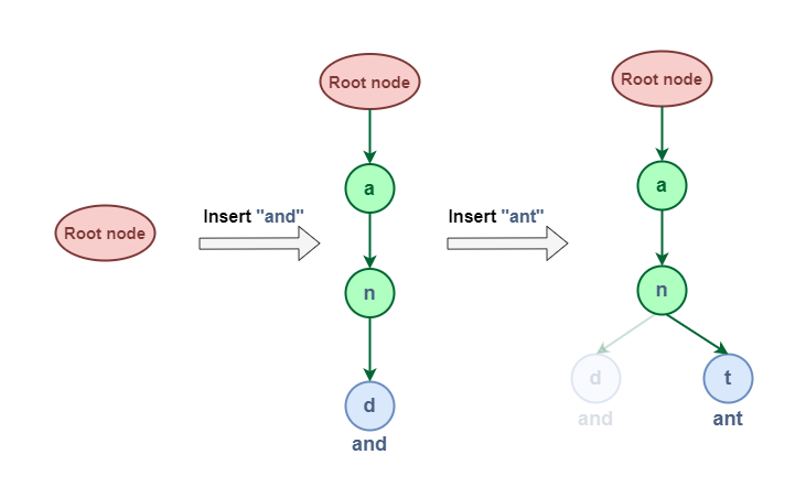
To insert a key to Trie, we need to do the following steps:
- Starting from the root, we check if the current node has a child corresponding to the first character of the key. If yes, we move to that child and continue to check the next character.
- If no, we create a new node and link it to the current node.
- We repeat the above steps until we reach the last character of the key. Then we mark the last node as the end of the key.
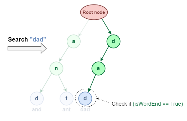
To search a key in Trie, we need to do the following steps:
- Starting from the root, we check if the current node has a child corresponding to the first character of the key. If yes, we move to that child and continue to check the next character.
- If no, we return
False. - We repeat the above steps until we reach the last character of the key. Then we return
Trueif the last node is marked as the end of the key.
def chartoIndex(ch):
    # private helper function
    # Converts key current character into index
    # use only 'a' through 'z' and lower case
    return ord(ch)-ord('a')

class Trie:

    def __init__(self):
        self.root = TrieNode()

    def insert(self, key):
        cur = self.root
        length = len(key)
        for level in range(length):
            index = chartoIndex(key[level])
            if not cur.children[index]:
                cur.children[index] = TrieNode()
            cur = cur.children[index]
        cur.isEndOfWord = True

    def search(self, key):
        cur = self.root
        length = len(key)
        for level in range(length):
            index = chartoIndex(key[level])
            if not cur.children[index]:
                return False
            cur = cur.children[index]
        return cur != None or cur.isEndOfWord
Another implementation of Trie is to use dictionary which is preferred in Leetcode.
class TrieNode:
    def __init__(self):
        self.children = dict()
        self.isEndOfWord = False

class Trie:
    def __init__(self):
        self.root = TrieNode()

    def insert(self, word):
        cur = self.root
        for ch in word:
            if ch not in cur.children:
                cur.children[ch] = TrieNode()
            cur = cur.children[ch]
        cur.isEndOfWord = True

    def search(self, word):
        cur = self.root
        for ch in word:
            if ch not in cur.children:
                return False
            cur = cur.children[ch]
        return cur != None or cur.isEndOfWord
Enjoy Reading This Article?
Here are some more articles you might like to read next: