Connection between Flatness and Generalization
In this post, I will try to answer the question: “Why does flatness correlate with generalization?” Specifically, we understand that a flat minimum is a solution with a low gradient norm around it, indicating that the loss function is flat (i.e., has a small gradient) with respect to the parameters around this solution. However, generalization is measured concerning the data distribution, not the parameters. So, why does a flat minimum correlate with generalization?
First, let’s clarify some concepts:
- Flatness or Sharpness: A flat minimum is a solution with a low gradient norm around it, meaning the loss function is flat (small gradient) with respect to the parameters around the solution. The flatness of a minimum can be defined as the ratio of the largest to the smallest eigenvalue of the Hessian matrix at the minimum.
- Generalization: Generalization is the ability of a model to perform well on unseen data. It is important to note that generalization is usually mentioned concerning the data distribution, not the parameters. There are many types of unseen data, the most common being held-out test data, which is drawn from the same distribution as the training data. Other types of unseen data include out-of-distribution (OOD) data and adversarial examples. OOD data is drawn from a different distribution than the training data, for example, a model trained on pictures of cats and dogs might be tested on drawings of animals. Adversarial examples are intentionally or unintentionally perturbed inputs that cause a model to make incorrect predictions. According to [1], there are two types of adversarial examples: off-manifold adversarial examples, generated by adding small perturbations or noise to the input data (e.g., standard gradient-based attacks like PGD), and on-manifold adversarial examples, which are generated by more complex transformations so that they remain within the data distribution.
While flatness can be defined mathematically, the definition of generalization is still ambiguous to me.
Does DNNs generalize or memorize?
It is well known tha Deep Neural Networks (DNNs) are powerful models that can fit complex functions and perform well on unseen data on wide range of tasks. However, do DNNs really generalize or just memorize the training data? Surprisingly, there are many empirical evidences that show the latter.
DNNs can memorize perfectly
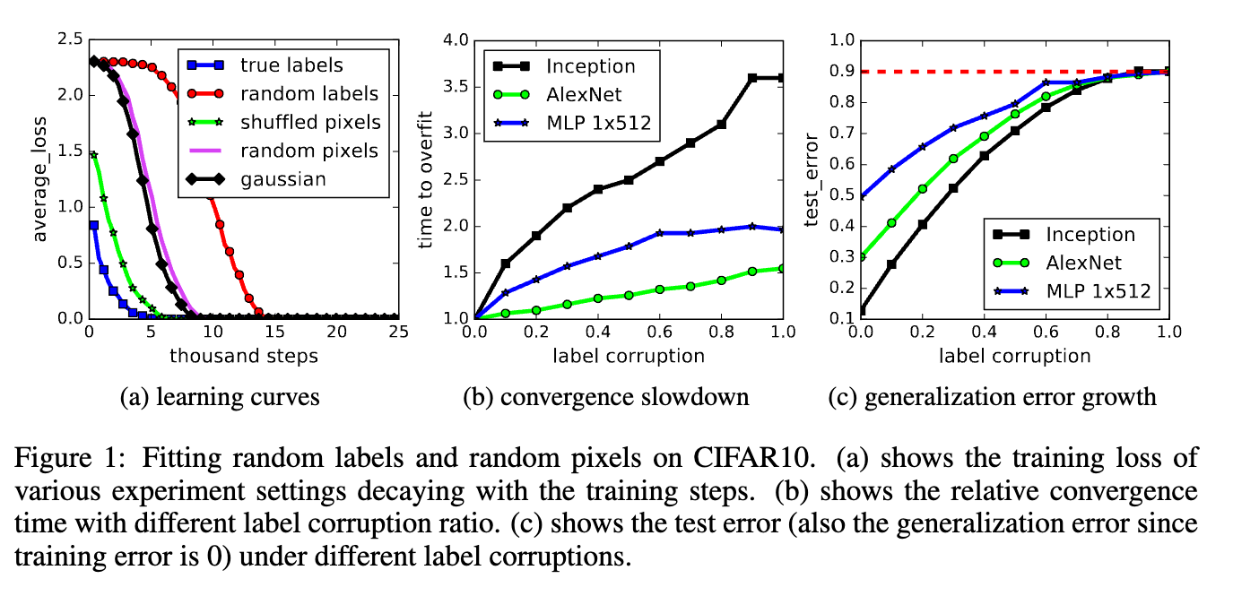
In this seminal paper [2], the authors argue that DNNs so powerful that they just memorize the training data but not generalize. They did a very interesting experiment to show that DNNs can easily fit the training data perfectly even under extreme scenarios, such as:
- Random labels: all the labels are replaced with random ones.
- Random pixels: a different random permutation is applied to each image independently.
Shortcuts learning
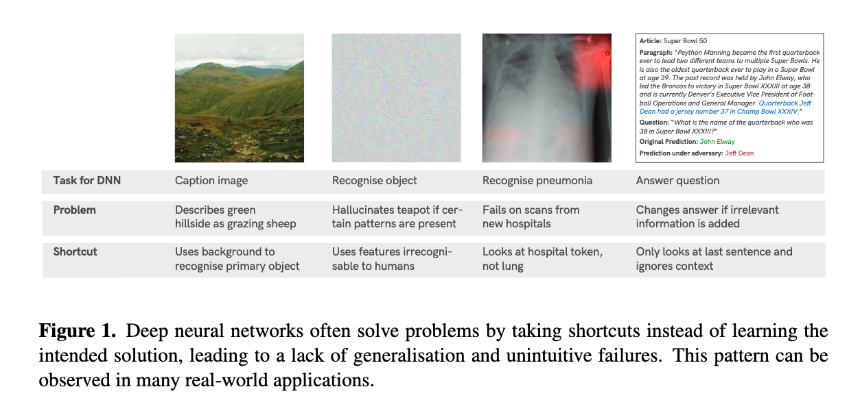
We acknowledge that DNNs can overfit but it is still surprising that they can fit the training data perfectly even under extreme scenarios. Continuing the intriguing memorization property of DNNs, in [4] the authors claim that yes, DNNs can learn to memorize the training data, but they first tend to exploit the simple patterns in the data first before memorizing the data. They also show that regularization techniques make the model harder to memorize noisy data. [5] also shows that DNNs tend to learn shortcuts (e.g., easy features or patterns) to solve the task rather than learning robust features (human interpretable features) that generalize well to unseen data.
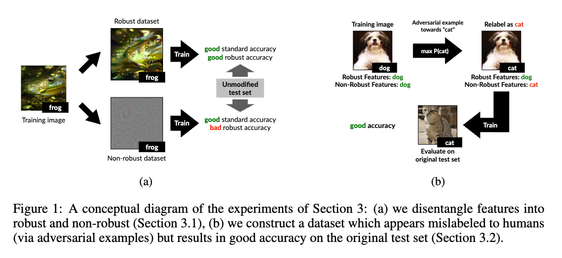
In [3], the authors also claim that DNNs tend to learn features that useful for the task but not necessarily the features that are human-interpretable. To prove this, they generated adversarial examples that are imperceptible to humans but can fool the DNNs, e.g., the image of a dog that is classified as a cat. Then they relabel these adversarial examples to the incorrect labels and retrain the model. Surprisingly, the model can still classify the test data correctly.
Information Theory Perspective
[7] brings a beautiful perspective to understand the generalization of DNNs from the information theory perspective. They argue that the generalization of DNNs can be understood by the information bottleneck principle, which states that the representation \(T\) should retain as much information about the input \(X\) as possible while being as informative as possible about the output \(Y\).
The process of information going through the layers of DNNs can be viewed as a Markov chain of information \(X \rightarrow T_1 \rightarrow T_2 \rightarrow \ldots \rightarrow T_k \rightarrow \hat{Y}\), where \(X\) is the input data, \(T_i\) is the representation at layer \(i\), and \(\hat{Y}\) is the output. By the chain rule of mutual information, we have
\[I(X;Y) \geq I(T_1;Y) \geq I(T_2;Y) \geq \ldots \geq I(T_k;Y) \geq I(\hat{Y};Y)\]which means that the information about the ground truth \(Y\) is decreasing as we go deeper into the network.
\[H(X) \geq I(X;T_1) \geq I(X;T_2) \geq \ldots \geq I(X;T_k) \geq I(X;\hat{Y})\]The information bottleneck principle [7] states that the representation \(T_i\) should retain as much information about the input \(X\) as possible while being as informative as possible about the output \(Y\).
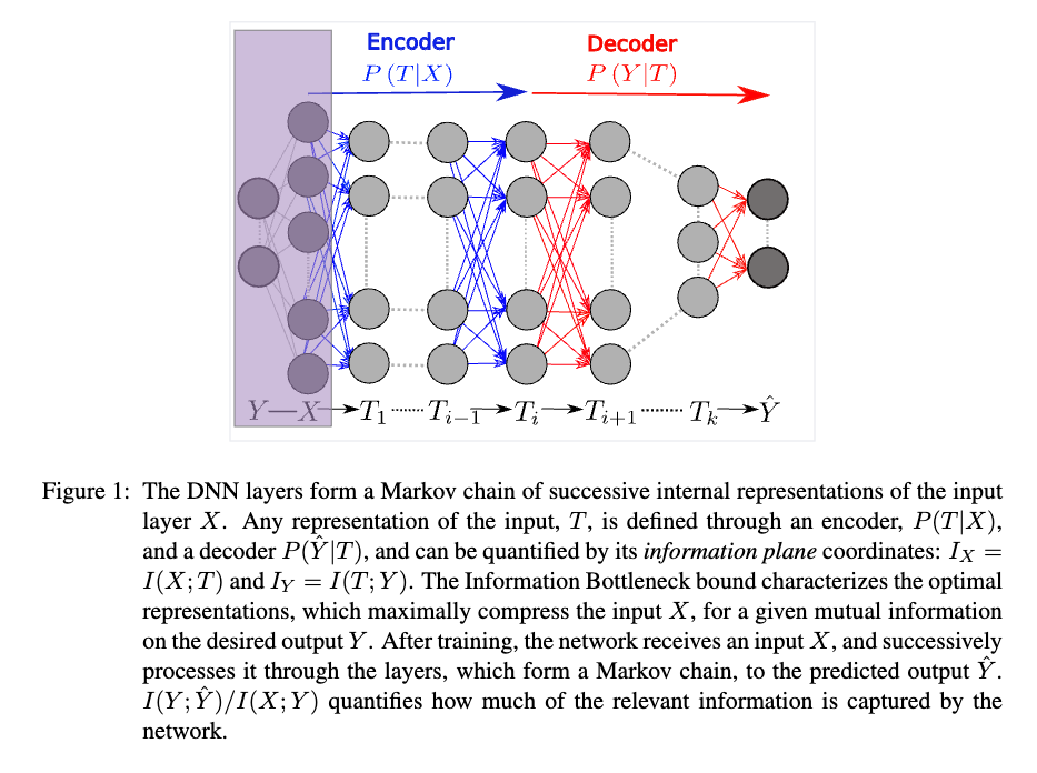
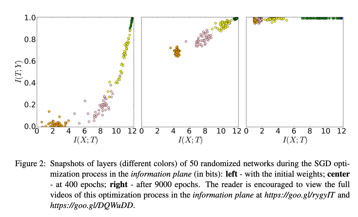
As in [7], the training process of DNNs can be divided into two phases: the fitting (or learning) phase and the forgetting phase. During the fitting phase, the model strives to fit the training data by capturing all available information. This is evidenced by the mutual information \(I(X, T)\) and \(I(T, Y)\) both increasing, indicating that the intermediate representations \(T\) are becoming more informative about the input data \(X\) or the output \(Y\).
In contrast, the forgetting phase involves the model discarding or ignoring irrelevant information that is not useful for the task, while retaining relevant information. This phase is characterized by a decrease in the mutual information \(I(X, T)\), while \(I(T, Y)\) is maintained. The model is effectively filtering out irrelevant information to focus on the task at hand. Again, as discussed above, the useful information is not necessarily the human-interpretable features but the features that are useful for the task.
Connection to Overfitting
As discussed in [7], the fitting phase is much faster than the forgetting phase, which means that the model can fit the training data quickly but it takes longer to forget the irrelevant information. The forgetting phase is also called as the representation compression phase or encoding phase, where the model compresses the input data into a more compact representation that is relevant to the task. While the increasing of \(I(T, Y)\) is expected from the cross-entropy loss minimization, the decreasing of \(I(X, T)\) is not trivial. And this is the result of standard SGD training, not a special regularization technique.
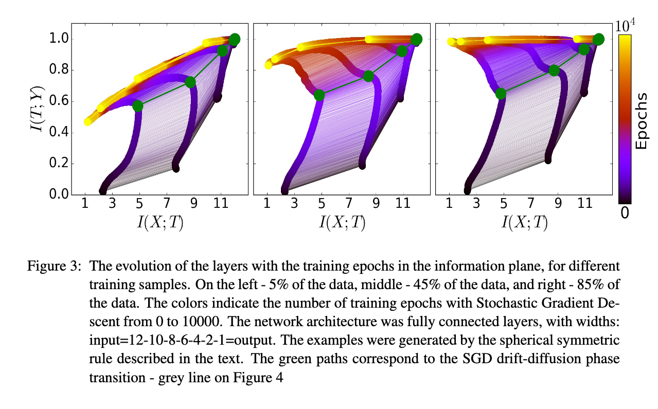
The left figure is the Information Plane of a model trained with a small dataset (5\%), which shows that the information about label \(I(Y,T)\) is significantly reduced during the forgetting phase, indicating the overfitting problem. This problem is not observed in the case of a large dataset (85\%), where the model can still retain the information about the label \(I(Y,T)\) during the forgetting phase. Note that the information about the input \(I(X,T)\) is still decreasing in both cases, which means that the model is still filtering out irrelevant information, and the overfitting problem mainly comes from the loss of information about the label \(I(Y,T)\) during the forgetting phase.
Side note: It is a worth-mentioning that the work in [7] is based on an assumption about the Markov chain of information in DNNs, which means that the information at layer \(i\) is only dependent on the information at layer \(i-1\). This assumption may not hold in modern DNNs, where skip connections, residual connections, and other complex architectures are used.
Connection between Flatness and Generalization
The question about “why does flatness correlate with generalization?” is actually non-trivial than it seems. Most the examplanation are based on the empirical observations or intuitions [8], rather than a rigorous theoretical proof.
The concept of sharp and flat minimizers have been discussed in the statistics and machine learning literature. [9] was one of the first to introduce the concept of flat minimizers, which the function varies slowly in a relatively large neighborhood. A flat minimum corresponds to weights many of which can be given with low precision, e.g., \(w_i = 0.1\) or \(w_i = 0.1001\) are almost equivalent, whereas a sharp minimum requires high precision. The connection between flat minimal and overfitting can be explained through the lens of the minimum description length (MDL) theory, which suggests that lower complexity models correspond to high generalization performance. Since flat minimizers can be specified with lower precision than to sharp minimizers, they tend to have better generalization performance. [8] show that large-batch training tends to converge to sharp minimizers, which are associated with poor generalization performance.
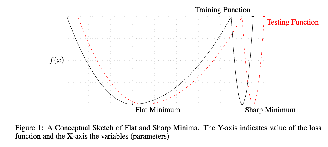
[10] proposed a new optimization algorithm called Sharpness-Aware Minimization (SAM) that aims to find flat minimizers by seeking out parameter values whose entire neighborhoods have uniformly low training loss value (equivalently, neighborhoods having both low loss and low curvature). The authors provided a generalization bound based on sharpness:
For any \(\rho>0\) and any distribution \(\mathscr{D}\), with probability \(1-\delta\) over the choice of the training set \(\mathcal{S}\sim \mathscr{D}\), \(\begin{equation} L_\mathscr{D}(\boldsymbol{w}) \leq \max_{\|\boldsymbol{\epsilon}\|_2 \leq \rho} L_\mathcal{S}(\boldsymbol{w} + \boldsymbol{\epsilon}) +\sqrt{\frac{k\log\left(1+\frac{\|\boldsymbol{w}\|_2^2}{\rho^2}\left(1+\sqrt{\frac{\log(n)}{k}}\right)^2\right) + 4\log\frac{n}{\delta} + \tilde{O}(1)}{n-1}} \end{equation}\) where \(n=|\mathcal{S}|\), \(k\) is the number of parameters and we assumed \(L_\mathscr{D}(\boldsymbol{w}) \leq \mathbb{E}_{\epsilon_i \sim \mathcal{N}(0,\rho)}[L_\mathscr{D}(\boldsymbol{w}+\boldsymbol{\epsilon})]\).
The bound shows that the generalization error \(L_\mathscr{D}(\boldsymbol{w})\) is upper bounded by the maximum training loss \(L_\mathcal{S}(\boldsymbol{w} + \boldsymbol{\epsilon})\) in a neighborhood of the parameters \(\boldsymbol{w}\). Therefore, when minimizing the right-hand side of the bound, the algorithm is encouraged to find flat minimas that has lower generalization error \(L_\mathscr{D}(\boldsymbol{w})\).
Controversy
While in some extent, the flatness of the loss function around the minimum can be a good indicator of generalization as shown in series of SAM papers [10], there are also some controversies pointed out the opposite. For example, [11] showed that flatness is sensitive to reparameterization and cannot be used as a reliable indicator of generalization. More specifically, reparameterization is a transformation of the parameters that does not change the function represented by the model, e.g., changing the scale of the weights or changing the way the latent variables are sampled in VAEs. In [11], the authors pointed out that we can reparameterize the model without chaining its outputs while making the sharp minima arbitrarily flat and vice versa.
[12] provided a more intuitive explanation of the disconnection between flatness and generalization. More specifically, if defining the sharpness of the loss function \(L\) as in the SAM paper [10]:
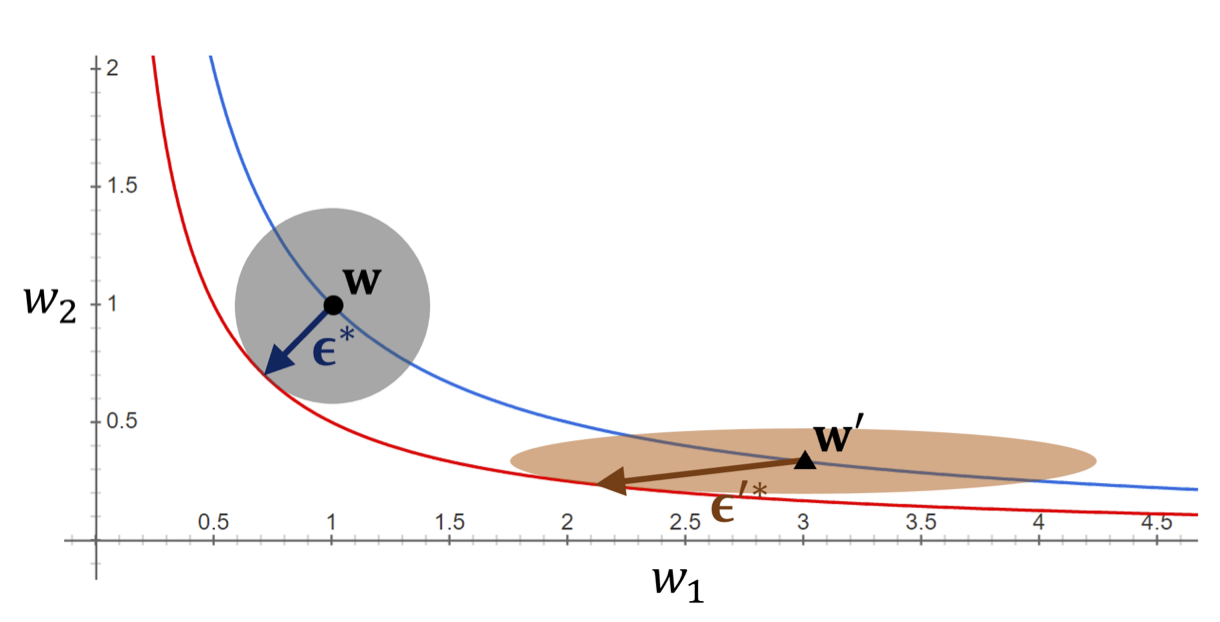
\[\begin{equation}\label{eq:s1} \max_{\Vert \boldsymbol{\epsilon} \Vert_{2} \leq \rho}L_S(\boldsymbol{w}+\boldsymbol{\epsilon}) - L_S(\boldsymbol{w}). \end{equation}\]As illustrated in the figure below, if we consider the loss function \(L_S(\boldsymbol{w})\) is a convex function of \(\boldsymbol{w}\) with only two parameters \(w_1\) and \(w_2\) so its loss surface can be represented in a 2D space. Then, if we assume that \(A\) is a scaling operator on the weight space that does not change the loss function, i.e., \(L_S(A\boldsymbol{w}) = L_S(\boldsymbol{w})\), so by varying the scaling factor of the weights, we can have a countour of the loss function that has the same value. Within this setting, we can see that while having the same loss value, the two model \(\boldsymbol{w}\) and \(A\boldsymbol{w}\) can have arbitrarily different sharpness values as defined in Eq. \eqref{eq:s1}, i.e.,
\[\max_{\Vert \boldsymbol{\epsilon} \Vert_{2} \leq \rho} L_S(\boldsymbol{w}+\boldsymbol{\epsilon}) \neq \max_{\Vert \boldsymbol{\epsilon} \Vert_{2} \leq \rho} L_S( A\boldsymbol{w}+\boldsymbol{\epsilon})\]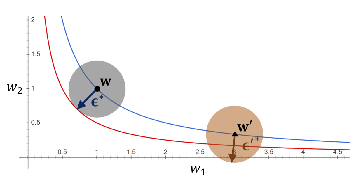
This means that the flatness of the loss function around the minimum is not necessarily correlated with generalization. And to mitigate this scaling dependency problem, the authors [12] proposed a new concept of adaptive sharpness-aware minimization (ASAM) that adaptively adjusts the sharpness of the loss function to make it invariant to scaling, i.e., instead of considering the sphere neighborhood of the parameters \(\Vert \boldsymbol{\epsilon} \Vert_{2} \leq \rho\) which takes every direction equally, the ASAM considers the ellipsoid neighborhood \(\Vert T^{-1}_\boldsymbol{w} \boldsymbol{\epsilon}\Vert _{p} \leq \rho\) where \(T^{-1}_\boldsymbol{w}\) is a normalization/weighted operator that makes the loss function invariant to scaling.
Conclusion
In this post, we have discussed the connection between flatness and generalization in DNNs. While flat minimizers are often associated with better generalization performance, there are also some controversies about the reliability of flatness as an indicator of generalization. The flatness of the loss function around the minimum can be a good indicator of generalization, but it is sensitive to reparameterization. More research is needed to better understand the relationship between flatness and generalization in DNNs.
References
[1] Stutz, David, Matthias Hein, and Bernt Schiele. “Disentangling adversarial robustness and generalization.” Proceedings of the IEEE/CVF Conference on Computer Vision and Pattern Recognition. 2019.
[2] Zhang, Chiyuan, et al. “Understanding deep learning (still) requires rethinking generalization.” Communications of the ACM 64.3 (2021): 107-115.
[3] Ilyas, Andrew, et al. “Adversarial examples are not bugs, they are features.” Advances in neural information processing systems 32 (2019).
[4] Arpit, Devansh, et al. “A closer look at memorization in deep networks.” International conference on machine learning. PMLR, 2017.
[5] Geirhos, Robert, et al. “Shortcut learning in deep neural networks.” Nature Machine Intelligence 2.11 (2020): 665-673.
[6] ‘How neural networks learn’ - Part III: Generalization and Overfitting by Arxiv Insights
[7] Shwartz-Ziv, Ravid, and Naftali Tishby. “Opening the black box of deep neural networks via information.” arXiv preprint arXiv:1703.00810 (2017).
[8] Keskar, Nitish Shirish, et al. “On large-batch training for deep learning: Generalization gap and sharp minima.” arXiv preprint arXiv:1609.04836 (2016).
[9] Hochreiter, Sepp, and Jürgen Schmidhuber. “Flat minima.” Neural computation 9.1 (1997): 1-42.
[10] Foret, Pierre, et al. “Sharpness-aware Minimization for Efficiently Improving Generalization.” International Conference on Learning Representations. 2021.
[11] Dinh, Laurent, et al. “Sharp minima can generalize for deep nets.” International Conference on Machine Learning. PMLR, 2017.
[12] Kwon, Jungmin, et al. “Asam: Adaptive sharpness-aware minimization for scale-invariant learning of deep neural networks.” International Conference on Machine Learning. PMLR, 2021.
Enjoy Reading This Article?
Here are some more articles you might like to read next: