Cold Diffusion - Inverting Arbitrary Image Transforms Without Noise
About the paper
- Accepted to NeurIPS 2023.
- From Tom Goldstein’s group at University of Maryland. Tom and his postdoc Micah Goldblum are two favorite leading researchers of mine. His group has published many interesting, creative and trendy (of course
 ) papers in the field of ML, particullary in Trustworthy Machine Learning. Recently, his group won the best paper award at ICML 2023 for the watermarking on LLM paper. So good.
 - Link to the paper: https://arxiv.org/abs/2208.09392
- Github: https://github.com/arpitbansal297/Cold-Diffusion-Models

Many papers on diffusion models primarily focus on the diffusion/degradation process through the addition of Gaussian noise. This method involves introducing small amounts of Gaussian noise to an image during the forward diffusion process, gradually resulting in a heavily noised image. Conceptually, this noising process can be likened to a random walk on a manifold if we consider the data space as such. The objective of a diffusion model is to effectively reverse this degradation process, aiming to reconstruct the original image from its noised version.
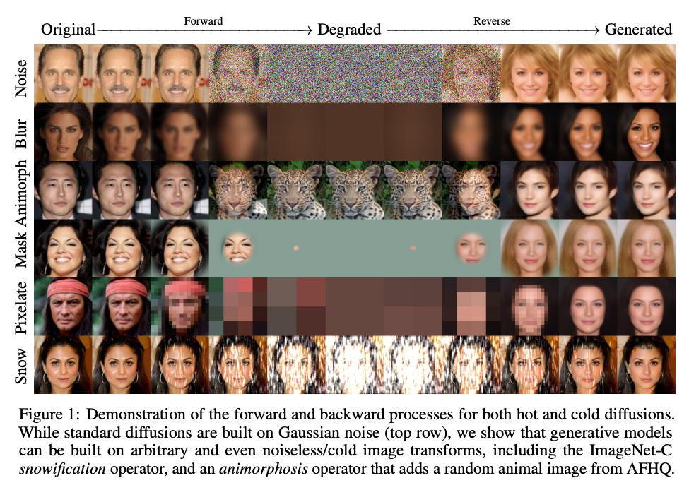
In this paper, the authors posed an intriguing question: “Can we replace the Gaussian noise in the degradation process with an image transformation operation, such as blurring, pixelation, or masking?”. Surprisingly, this work demonstrated that it is indeed possible. The authors proposed a generalized diffusion model, termed Cold Diffusion, that can employ arbitrary image transformations in the degradation process. The model is trained to invert these transformations and recover the original image. By using some generation tricks, the model not only can recover the original image but also can generate new/novel images. This work opens up a new direction for diffusion models, allowing them to be applied to a broader range of image transformations beyond Gaussian noise.
Method
What is the cold diffusion model?
The proposed cold diffusion model presents a straightforward mathematical formulation (I still wonder why they called it “cold” ![]() ).
Given an input image \(x\) and a transformation function \(D\), the reverse process is parameterized by a neural network \(R_\theta\):
).
Given an input image \(x\) and a transformation function \(D\), the reverse process is parameterized by a neural network \(R_\theta\):
To train the standard diffusion models such as DDPM, the high level idea is to match the predicted noise with the true noise added at particular diffusion step. However, in the cold diffusion model, the above objective is actually more similar to the autoencoder, i.e., the model is trained to minimize the difference between the input image and the recovered image. The difference to the autoencoder is that the degradation process is done by a transformation function \(D\) not by an encoder, and more importantly, is done through a series of steps, not just one step. To me, the more similar to the diffusion model might be the paper Soft Diffusion: Score Matching for General Corruptions.
How to sampling?

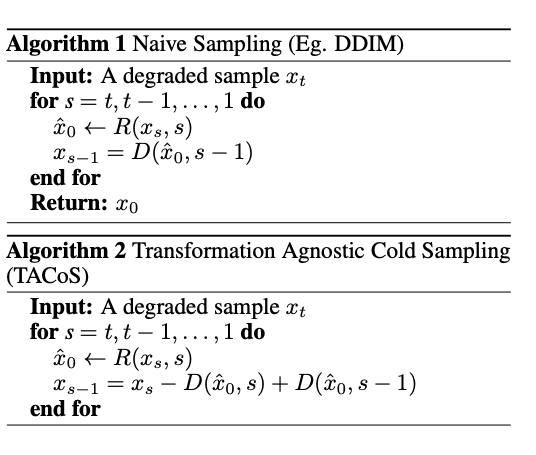
Naively, after training the cold diffusion model, we can sample the image as the algorithm 1 above, i.e., at each step, we apply diffusion inversion (read more about it here) to predict the original image from current step \(\hat{x}_0 = R(x_s, s)\), then apply the transformation function \(D\) to get the next step \(x_{s-1} = D(\hat{x}_0, s-1)\), and so on. It is worth noting that in the standard diffusion model, the initial image \(x_T\) is sampled from a Gaussian distribution; however, in this cold diffusion model, the initial image (they called it “a degraded sample”) is sampled from the final step of the degradation process, i.e., \(x_T = D(x_0, T)\). It is make sense to me because there is no mathematical formulation for the degradation process unlike as in the standard one, where \(x_T \sim \mathcal{N}(0, I)\). (Refer to Section 5.2 in the paper).
So the author proposed some tricks to improve the sampling process:
- Using Algorithm 2 instead of Algorithm 1 to mitigate the compounding error from the imperfect inversion function \(R_\theta\). It is based on the approximation \(D(x,s) \approx x + s . e(x) + HOT\), where \(e(x)\) is the gradient of the transformation function \(D\) at \(x\), but be considered as a constant vector (not dependent on \(s\), questionable to me). The HOT term is the higher order terms that can be ignored. But this trick is just to help the recovery process, not the generation or introducing better diversity/novelty to the generated images.
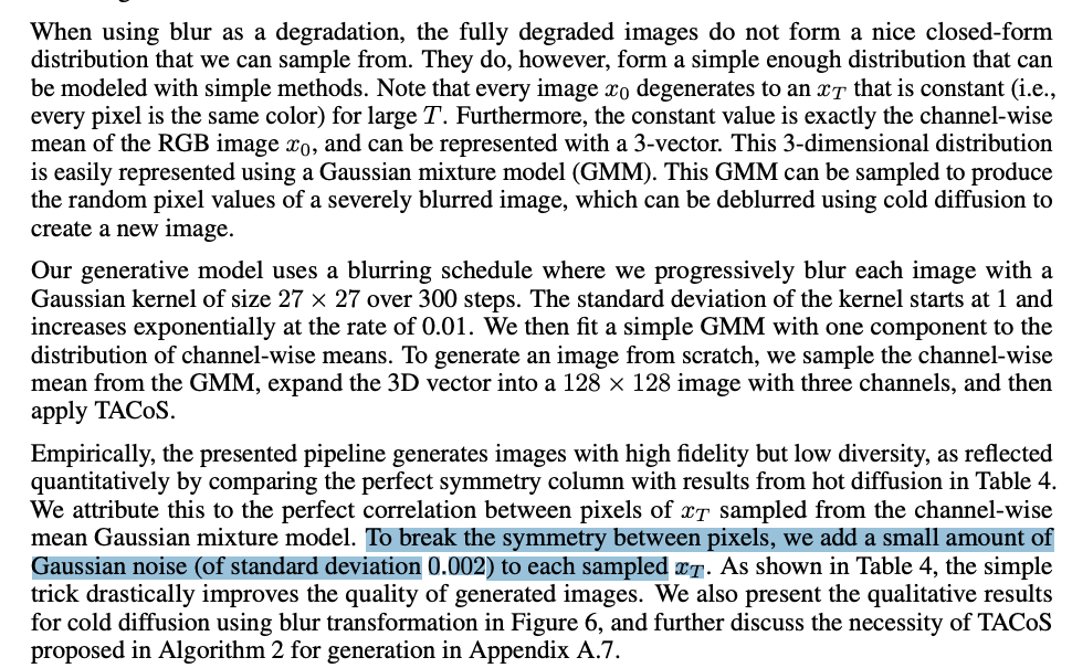
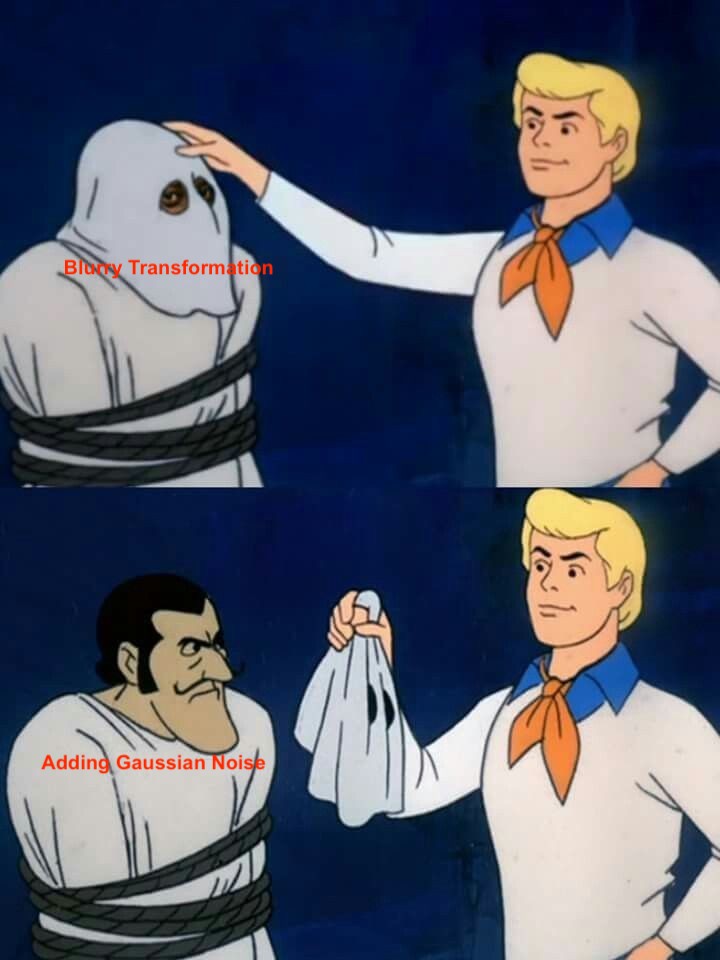
- The key trick to improve the diversity is to add a small amount of noise in each sample \(x_T\).


Reflection/Thoughts
So after the success of this paper, we might ask “What is the core of the diffusion model that makes it work?” To me, there are few key components:
- The two opposite processes: degradation and recovery. Interestingly, the degradation process can be done by a wide range of operations, even with animorphosis operators, that adds a random animal image to the original image. At the end of the degradation process, the image is still a valid image (clean and clear under human eyes). Therefore, to me, the final goal of the degradation process is to remove totally the information of the original image, not to make the image unrecognizable (nothing to do with human preception here). Mathematically, \(I(x, D(x,t)) \to 0\) when \(t\) becomes larger, where \(I\) is the mutual information between \(x\) and \(D(x,t)\).
- The iterative process: the diffusion/degradation process is done through a series of steps, not just one step.
- What is the source of stochasticity which decides the novelty of the generated images?
Enjoy Reading This Article?
Here are some more articles you might like to read next: