Papers Reading
- One-dimensional Adapter to Rule Them All - Concepts, Diffusion Models and Erasing Applications
- Universal and Transferable Adversarial Attacks on Aligned Language Models
- Cold Diffusion: Inverting Arbitrary Image Transforms Without Noise
- Your Diffusion Model is Secretly a Zero-Shot Classifier
- Rethinking Conditional Diffusion Sampling with Progressive Guidance
- A new perspective on the motivation of VAE (by Dinh)
- FLOW MATCHING FOR GENERATIVE MODELING (ICLR 2023)
- Diffusion Models Beat GANs on Image Synthesis
- TRADING INFORMATION BETWEEN LATENTS IN HIERARCHICAL VARIATIONAL AUTOENCODERS
One-dimensional Adapter to Rule Them All - Concepts, Diffusion Models and Erasing Applications
- Project page: https://github.com/AtsuMiyai/UPD/

Motivation:
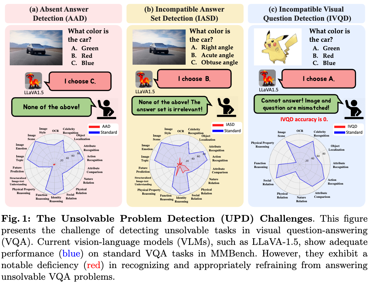
- With the development of powerful foundation Vision-Language Models (VLMs) such as the LLaVA-1.5 model, we can now solve visual question-answering (VQA) quite well by simply plugging the foundation VLMs as zero-shot learners (i.e., no need for fine-tuning on the VQA task).
- However, similar to the hallucination in LLMs, when the LLMs confidently provide false answers, the VLMs also face the hallucination problem when they always provide answers from a given answer set even when these questions are unsolvable (a very important point: unsolvable with respect to a given answer set).
- To systematically benchmark the problem, the authors proposed three new challenges/types of unsolvable problems: Absent Answer Detection (AAD), Incompatible Answer Set Detection (IASD), and Incompatible Visual Question Detection (IVQD).
- Note that these problems are not open-ended problems, but closed ones, i.e., the answer is limited within a given answer set. Moreover, the answer set designed by the authors does not completely cover the answer space, i.e., lacking answers like “None of the above” or “I don’t know,” making the problem become unsolvable with respect to the given answer set.
- With the proposed unsolvable problems, the VLMs like GPT-4 likely provide hallucination answers, so that the authors can evaluate the trustworthiness of the VLMs.One-dimensional Adapter to Rule Them All - Concepts, Diffusion Models and Erasing Applications
Universal and Transferable Adversarial Attacks on Aligned Language Models
- Link to the blog post: https://tuananhbui89.github.io/blog/2024/paper-llm-attacks/
Cold Diffusion: Inverting Arbitrary Image Transforms Without Noise
- Link to the blog post: https://tuananhbui89.github.io/blog/2024/paper-cold-diffusion/
Your Diffusion Model is Secretly a Zero-Shot Classifier
- Accepted to ICCV 2023.
- Affiliation: CMU.
- Github: https://github.com/diffusion-classifier/diffusion-classifier
Motivations:
- Diffusion models such as Stable Diffusion are trained with self-supervised learning, i.e., \((x,y)\), with \(y\) is the label of \(x\), such as an image’s caption.
- Question: Can we use a pre-trained DM to estimate \(p(y \mid x)\)?
Proposed Method:
In general, classification using a conditional generative model can be done by using Bayes’ theorem:
\[p_\theta (c_i \mid c) = \frac{p(c_i) p_\theta(x \mid c_i)}{\sum_j p(c_j) p_\theta (x \mid c_j)}\]where \(c_i\) is the class label of \(x\), prior \(p(c)\) over labels \(\{ c_i \}\).
However, obtain posterior distribution \(p_\theta (c_i \mid x)\) over set of labels \(\{ c_i \}\) is intractable.
\[p_\theta (c_i \mid x) = \frac{\exp{ \{ - \mathbb{E}_{t,\epsilon} \| \epsilon - \epsilon_\theta (x_t, c_i) \| } \} }{\sum_j \exp{ \{ - \mathbb{E}_{t,\epsilon} \| \epsilon - \epsilon_\theta (x_t, c_j) \| } \} }\]Why is it intractable? Because the expectation \(\mathbb{E}_{t,\epsilon}\) is over the diffusion process, which is intractable / expensive to compute.
Therefore, the authors propose to use the following approximation:
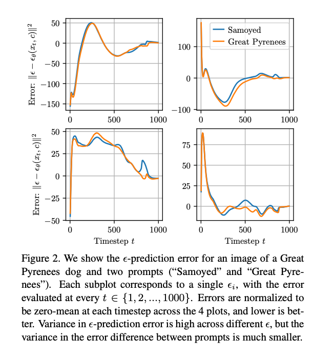
\[p_\theta (c_i \mid x) \approx \frac{1}{\sum_j \exp \{ \mathbb{E}_{t,\epsilon} \left[ \| \epsilon - \epsilon_\theta (x_t, c_i) \|^2 - \| \epsilon - \epsilon_\theta (x_t, c_j) \|^2 \right] \}}\]Why is it cheaper? Because using the above approximation, we only need to compute the difference between each pair of \(c_i\) and \(c_j\). To support this approximation, the authors measured the error score \(\| \epsilon - \epsilon_\theta(x_t, c_i) \|\) for four different \(\epsilon\) and varying \(t\) and found that the error pattern is dependent on \(\epsilon\), and the difference between the error scores of two classes seems to be independent of \(\epsilon\) (ref. Figure 2)

Comparing the computational cost: Given one query image \(x\) and total \(C\) classes:
- The cost of the exact posterior \(p_\theta (c_i \mid x)\) is: \(C\) times of the cost to compute \(\mathbb{E}_{t,\epsilon} \| \epsilon - \epsilon_\theta (x_t, c_i) \|\). To compute \(\mathbb{E}_{t,\epsilon} \| \epsilon - \epsilon_\theta (x_t, c_i) \|\), we need to sample \(N\) pairs of \((t, \epsilon)\). Therefore, the cost is \(O(C N)\).
- The cost of the approximate posterior: also \(C\) times of the cost to compute \(\mathbb{E}_{t,\epsilon} [ \| \epsilon - \epsilon_\theta (x_t, c_i) \|^2 - \| \epsilon - \epsilon_\theta (x_t, c_j) \|^2 ]\).
Given the above analysis, I can see that the advantage of the approximation is not computational cost but the ability to compute the posterior distribution more accurately.
Some promising directions:
- Using more straight diffusion models such as Flow Straight and Fast: Learning to Generate and Transfer Data with Rectified Flow or Consistency models to accelerate the computation of the posterior.
Rethinking Conditional Diffusion Sampling with Progressive Guidance
Increase the diversity of classifier guidance paper by introduing a new technique called Progressive Guidance. In the DDPM model
\[x_{t-1} = \frac{1}{\sqrt{\alpha_t}} \left( x_t - \frac{1-\alpha_t}{\sqrt{1 - \bar{\alpha}_t} \epsilon_\theta (x_t, t)} \right) + \sigma_t z\]where \(z\) is a random noise. In the classifier guidance
\[x_{t-1} = \frac{1}{\sqrt{\alpha_t}} \left( x_t - \frac{1-\alpha_t}{\sqrt{1 - \bar{\alpha}_t} \epsilon_\theta (x_t, t)} \right) + \sigma_t z + s \sigma_t^2 \nabla_{x_t} \log p_\phi (y_c \mid x_t)\]Their proposed method:
\[x_{t-1} = \frac{1}{\sqrt{\alpha_t}} \left( x_t - \frac{1-\alpha_t}{\sqrt{1 - \bar{\alpha}_t} \epsilon_\theta (x_t, t)} \right) + \sigma_t z + w * \sum_{i=1}^c s_i \sigma_t^2 \nabla_{x_t} \log p_\phi (y_i \mid x_t)\]with \(s_i \geq 0\) is the degree of information injected into the sampling process by class \(y_i\).
Their intuition:
- By incorporating gradients from other classes during sampling, the conflict between the sampling and discriminative objectives can be decreased, resulting in diverse generated samples
- Using other classes’ gradients beyond the conditional class gradient helps avoid adversarial effects
What is adversarial effects? In the formulation of classifier guidance, the guidance signal is quite similar as in adversarial perturbation so that the perturbation is making nonsense to human eyes, however, it is still classified as the target class.
One important point of this paper is how to choose vector \(s\). They propose to model the correlation between labels via the description text of labels as follows:
- utilize ChatGPT to generate text descriptions for each class, e.g., class “dog” is described as “a domesticated carnivorous mammal that typically has a long snout, an acute sense of smell, nonretractable claws, and a barking, howling, or whining voice.”
- After removing stop words and other preprocessing text, we use a CLIP model to obtain each class’s embedding information \(v_i\).
- The embedding information is then utilized to calculate the similarity based on cosine similarity \(sim_{i,j} = \frac{v_i v_j}{\mid v_i \mid \mid v_j \mid}\).
- Given the conditional label c, we have the information degree for each label \(s_i = \frac{sim_{c,i}}{\sum_{j=1}^C sim_{c,j}} \; \forall 1 \leq i \leq C\).
Given starting vector \(s\), they also propose a strategy to update \(s\) during sampling process to make the vector \(s\) becomes more one-hot vector (with the highest value is the target class). The speed of updating is controlled by a hyperparameter \(\gamma\). It can be seen from Table 5 in the paper, if \(\gamma=0\) means that there is no update, the performance is very poor. However, if \(\gamma\) large means that the vector \(s\) is become more one-hot vector fast and keep it that way through the sampling process, the performance is also not good.
In Table 6, they also show the importance of starting vector \(s\), if \(s\) is from label smoothing or uniform distribution, the performance is not good as using the CLIP embedding.
A new perspective on the motivation of VAE (by Dinh)
- Assume that \(x\) was generated from \(z\) through a generative process \(p(x \mid z)\).
- Before observing \(x\), we have a prior belief about \(z\), i.e., \(z\) can be sampled from a Gaussian distribution \(p(z) = \mathcal{N}(0, I)\).
- After observing \(x\), we want to correct our prior belief about \(z\) to a posterior belief \(p(z \mid x)\).
- However, we cannot directly compute \(p(z \mid x)\) because it is intractable. Therefore, we use a variational distribution \(q(z \mid x)\) to approximate \(p(z \mid x)\). The variational distribution \(q(z \mid x)\) is parameterized by an encoder \(e(z \mid x)\). The encoder \(e(z \mid x)\) is trained to minimize the KL divergence between \(q(z \mid x)\) and \(p(z \mid x)\). This is the motivation of VAE.
Mathematically, we want to minimize the KL divergence between \(q_{\theta} (z \mid x)\) and \(p(z \mid x)\):
\[\mathcal{D}_{KL} (q_{\theta} (z \mid x) \parallel p(z \mid x) ) = \mathbb{E}_{q_{\theta} (z \mid x)} \left[ \log \frac{q_{\theta} (z \mid x)}{p(z \mid x)} \right] = \mathbb{E}_{q_{\theta} (z \mid x)} \left[ \log q_{\theta} (z \mid x) - \log p(z \mid x) \right]\]Applying Bayes rule, we have:
\[\mathcal{D}_{KL} (q_{\theta} (z \mid x) \parallel p(z \mid x) ) = \mathbb{E}_{q_{\theta} (z \mid x)} \left[ \log q_{\theta} (z \mid x) - \log p(x \mid z) - \log p(z) + \log p(x) \right]\] \[\mathcal{D}_{KL} (q_{\theta} (z \mid x) \parallel p(z \mid x) ) = \mathbb{E}_{q_{\theta} (z \mid x)} \left[ \log q_{\theta} (z \mid x) - \log p(x \mid z) - \log p(z) \right] + \log p(x)\] \[\mathcal{D}_{KL} (q_{\theta} (z \mid x) \parallel p(z \mid x) ) = - \mathbb{E}_{q_{\theta} (z \mid x)} \left[ \log p(x \mid z) \right] + \mathcal{D}_{KL} \left[ q_{\theta} (z \mid x) \parallel p(z) \right] + \log p(x)\]So, minimizing \(\mathcal{D}_{KL} (q_{\theta} (z \mid x) \parallel p(z \mid x) )\) is equivalent to maximizing the ELBO: \(\mathbb{E}_{q_{\theta} (z \mid x)} \left[ \log p(x \mid z) \right] - \mathcal{D}_{KL} \left[ q_{\theta} (z \mid x) \parallel p(z) \right]\).
Another perspective on the motivation of VAE can be seen from the development of the Auto Encoder (AE) model.
- The AE model is trained to minimize the reconstruction error between the input \(x\) and the output \(\hat{x}\).
- The AE process is deterministic, i.e., given \(x\), the output \(\hat{x}\) is always the same.
- Therefore, the AE model does not have contiguity and completeness properties as desired in a generative model.
- To solve this problem, we change the deterministic encoder of the AE model to a stochastic encoder, i.e., instead of mapping \(x\) to a single point \(z\), the encoder maps \(x\) to a distribution \(q_{\theta} (z \mid x)\). This distribution should be close to the prior distribution \(p(z)\). This is the motivation of VAE.
FLOW MATCHING FOR GENERATIVE MODELING (ICLR 2023)
- Link to the paper: https://openreview.net/pdf?id=PqvMRDCJT9t
- Link to my blog post: https://tuananhbui89.github.io/blog/2023/flowmatching/
Diffusion Models Beat GANs on Image Synthesis
Link to blog post
TRADING INFORMATION BETWEEN LATENTS IN HIERARCHICAL VARIATIONAL AUTOENCODERS
- published on ICLR 2023.
Revisit Rate-Distortion trade-off theory:
- Problem setting of Rate-Distortion trade-off
- How to learn a “useful” representation of data for downstream tasks?
- Using powerful encoder-decoder such as VAE, PixelCNN, etc. can easily ignore \(z\) and still obtain high marginal likelihood \(p(x \mid \theta)\). Therefore, we need to use a regularization term to encourage the encoder to learn a “useful” representation of \(z\), for example, as in Beta-VAE.
Rate distortion theory?
\[H - D \leq I(z,x) \leq R\]where \(H\) is the entropy of data \(x\) and \(D\) is the distortion of the reconstruction \(x\) from \(z\). \(R\) is the rate of the latent code \(z\) (e.g., compression rate).
\(R = \log \frac{e(z \mid x)}{m(z)}\) where \(e(z \mid x)\) is the encoder and \(m(z)\) is the prior distribution of \(z\). The higher the rate, the more information of \(x\) is preserved in \(z\). However, if the rate is high, it lessen the generalization ability of the \(\log p(x \mid z, \theta)\).
The mutual information has upper bound by the rate of the latent code \(z\). For example, if \(R=0\) then \(I(z,x)=0\). This is because \(e(z \mid x) = m(z)\), which means that the encoder cannot learn anything from the data \(x\).
Motivation of the paper:
- Reconsider the rate distortion theory in the context of hierarchical VAEs where there are multiple levels of latent codes \(z_1, z_2, \dots, z_L\).
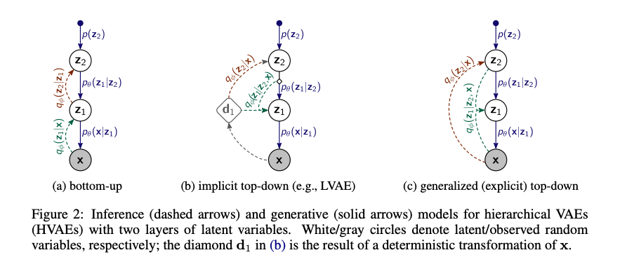
- The authors proposed a direct links between the input \(x\) and the latent codes \(z_1, z_2, \dots, z_L\). With this architecture, they can decompose the total rate to the rate of each latent code \(z_1, z_2, \dots, z_L\). Unlike the standard hierarchical VAEs, where the rate of each latent code is not directly related to the input \(x\) but the previous latent code \(z_{l-1}\).
- Then they can control the rate of each latent code.
Standard hierarchical VAEs:

Generalized Hierarchical VAEs:

Enjoy Reading This Article?
Here are some more articles you might like to read next: